Additional ARCH Models
In addition to the standard GARCH specification, EViews lets you perform estimation assuming a number of models of the variance. These include Integrated GARCH (IGARCH), Threshold ARCH (TARCH or GJRARCH), Exponential GARCH (EGARCH), Power ARCH (PARCH), component GARCH (CGARCH), Fractionally Integrated GARCH and EGARCH (FIGARCH and FIEGARCH), and Mixed Data Sampling GARCH (MIDAS GARCH)
For many of these models, the user has the ability to choose the order, if any, of asymmetry.
The Integrated GARCH (IGARCH) Model
If one drops the constant term and restricts the remaining parameters of the variance specification to sum to one,
 | (27.19) |
such that
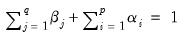 | (27.20) |
which gives an integrated GARCH specification. This model was originally described in Engle and Bollerslev (1986). To estimate this model, select IGARCH in the Restrictions drop-down menu for the GARCH/TARCH model.
The Threshold GARCH (TARCH or GJR-GARCH) Model
Threshold ARCH and Threshold GARCH (TARCH or GJR-GARCH) were introduced independently by Zakoïan (1994) and Glosten, Jaganathan, and Runkle (1993). The generalized specification for the conditional variance is given by:
 | (27.21) |
where

if

and 0 otherwise.
In this model, good news,

, and bad news.

, have differential effects on the conditional variance; good news has an impact of

, while bad news has an impact of

. If

, bad news increases volatility, and we say that there is a
leverage effect for the
i-th order. If

, the news impact is asymmetric.
Note that GARCH is a special case of the TARCH model where the threshold order

is set to zero. To estimate a TARCH model, specify your GARCH model with ARCH and GARCH order and then change the to the desired value.
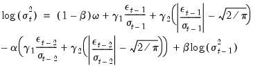
The Exponential GARCH (EGARCH) Model
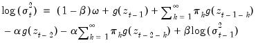
The EGARCH or Exponential GARCH model was proposed by Nelson (1991). The specification for the conditional variance is:
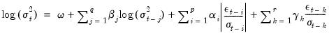 | (27.22) |
Note that the left-hand side is the
log of the conditional variance. This implies that the leverage effect is exponential, rather than quadratic, and that forecasts of the conditional variance are guaranteed to be nonnegative. The presence of leverage effects can be tested by the hypothesis that

. The impact is asymmetric if

.
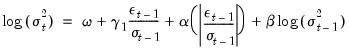
There are two differences between the EViews specification of the EGARCH model and the original Nelson model. First, Nelson assumes that the

follows a Generalized Error Distribution (GED), while EViews offers you a choice of normal, Student’s
t-distribution, or GED. Second, Nelson's specification for the log conditional variance is a restricted version of:
which is an alternative parameterization of the specification above. Estimating the latter model will yield identical estimates to those reported by EViews except for the intercept term

, which will differ in a manner that depends upon the distributional assumption and the order

. For example, in a

model with a normal distribution, the difference will be

.
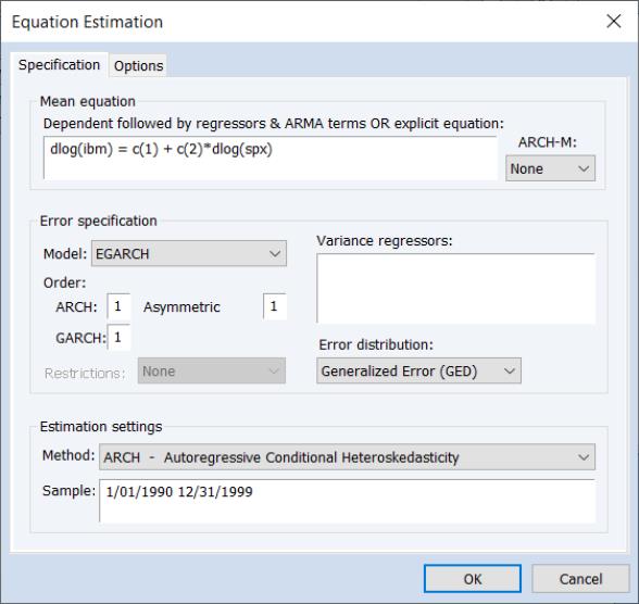
To estimate an EGARCH model, simply select the in the model specification dropdown menu and enter the orders for the , and the .
Notice that we have specified the mean equation using an explicit expression. The use of the explicit expression here is for illustration purposes only; since the expression is linear in the regressors, we could just as well have entered “dlog(ibm) c dlog(spx)” as our specification.
The Power ARCH (PARCH) Model
Taylor (1986) and Schwert (1989) introduced the standard deviation GARCH model, where the standard deviation is modeled rather than the variance. This model, along with several other models, is generalized in Ding
et al. (1993) with the Power ARCH specification. In the Power ARCH model, the power parameter

of the standard deviation can be estimated rather than imposed, and the optional

parameters are added to capture asymmetry of up to order

:
 | (27.23) |
where

,

for

,

for all

, and

.
The symmetric model sets

for all

. Note that if

and

for all

, the PARCH model is simply a standard GARCH specification. As in the previous models, asymmetric effects are present if

.
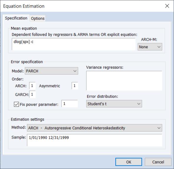
To estimate this model, simply select the PARCH in the model specification dropdown menu and input the orders for the , and terms. EViews provides you with the option of either estimating or fixing a value for

. To estimate the Taylor-Schwert's model, for example, you will to set the order of the asymmetric terms to zero and will set

to 1.
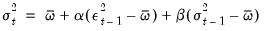
The Component GARCH (CGARCH) Model
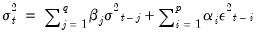
The conditional variance in the GARCH(1, 1) model:
 | (27.24) |
shows mean reversion to

, which is a constant for all time. By contrast, the component model allows mean reversion to a varying level

, modeled as:
 | (27.25) |
Here

is still the volatility, while

takes the place of

and is the time varying long-run volatility. The first equation describes the transitory component,

, which converges to zero with powers of (

). The second equation describes the long run component

, which converges to

with powers of

.

is typically between 0.99 and 1 so that

approaches

very slowly. We can combine the transitory and permanent equations and write:
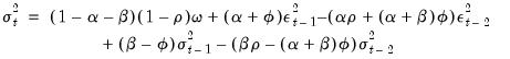 | (27.26) |
which shows that the component model is a (nonlinear) restricted GARCH(2, 2) model.
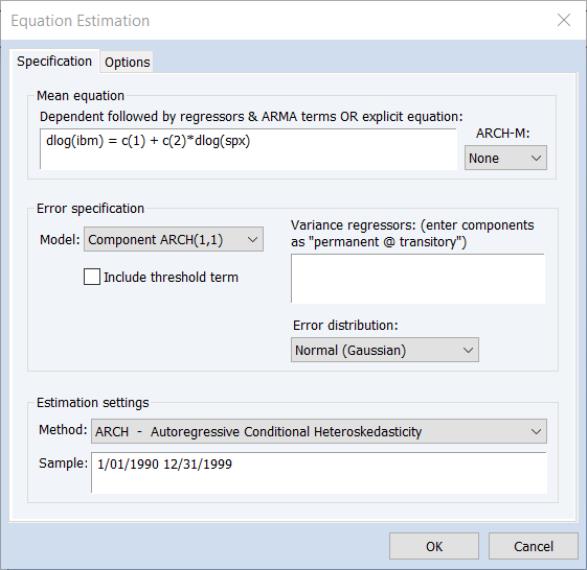
To select the Component ARCH model, simply choose in the dropdown menu. You can include exogenous variables in the conditional variance equation of component models, either in the permanent or transitory equation (or both). The variables in the transitory equation will have an impact on the short run movements in volatility, while the variables in the permanent equation will affect the long run levels of volatility.
An asymmetric Component ARCH model may be estimated by checking the checkbox. This option combines the component model with the asymmetric TARCH model, introducing asymmetric effects in the transitory equation and estimates models of the form:
 | (27.27) |
where

are the exogenous variables and

is the dummy variable indicating negative shocks.

indicates the presence of transitory leverage effects in the conditional variance.
Fractionally Integrated GARCH and EGARCH (FIGARCH)
EViews estimates Fractionally Integrated GARCH (FIGARCH) models, with support for both standard FIGARCH and Fractionally Integrated Exponential GARCH (FIEGARCH) specifications. The following discussion outlines the basic model and the interactive tools for estimating and working with FIGARCH models.
The Fractionally Integrated GARCH (FIGARCH) Model
While traditional GARCH models focus on short term dynamics of conditional variance, the fractionally integrated GARCH model (FIGARCH) model, introduced by Baillie, Bollerslev and Mikkelsen (1996, BBM), is designed to capture long run dependence properties of the variance.
Background
A standard GARCH model’s specification of the variance may be written as,
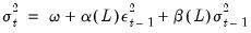 | (27.28) |
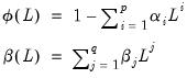
where

and

represent polynomial lags,
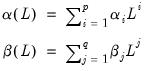 | (27.29) |
and

is the lag operator.
The fractionally integrated GARCH (FIGARCH) model modifies this specification by introducing a fractional difference term. The FIGARCH variance may be written as,
 | (27.30) |
where
 | (27.31) |
and

is the infinite lag operator
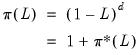 | (27.32) |
which uses the infinite lag expansion
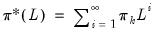 | (27.33) |
In practice, the infinite lag expansion is truncated to a finite number. For example, BBM suggest truncation at 1000 lags.
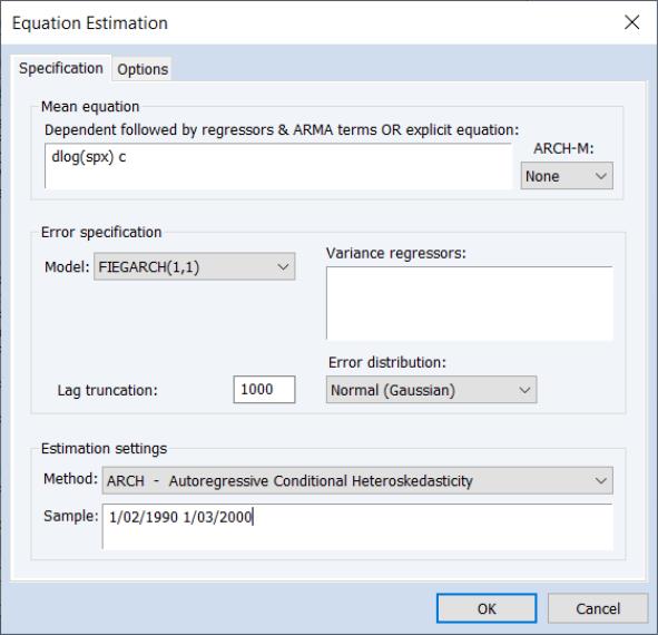
Estimating a FIGARCH model
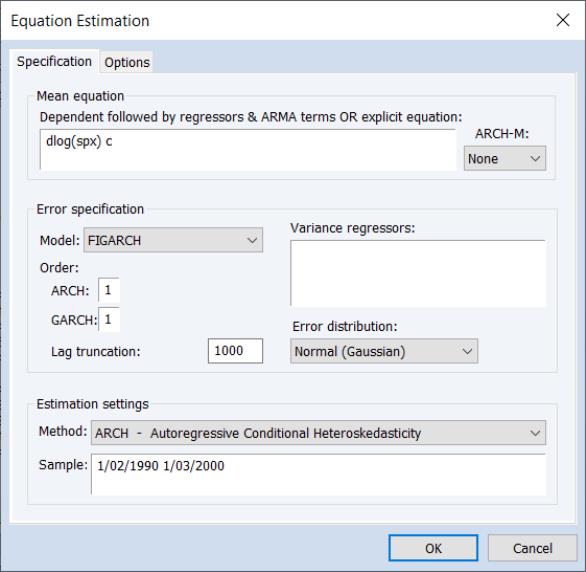
To estimate a FIGARCH model, select in the dropdown at the bottom of the dialog to display the GARCH dialog, then, in the section, choose in the dropdown menu:
As in other GARCH models, in the section of the dialog, you should enter your variables or explicit equation and select your specification.
You may select the and orders, list any , and select the .
Lastly, you may specify the FIGARCH number of terms in the FIGARCH infinite lag specification.
The Fractionally Integrated Exponential GARCH (FIEGARCH) Model
The FIEGARCH model of Bollerslev and Mikkelsen (1996) adds FIGARCH long-memory innovations to EGARCH processes.
Background
Before proceeding, note that while FIEGARCH models can be specified for arbitrary ARCH and GARCH orders, researchers typically restrict both to a single lag, and EViews currently supports only these FIEGARCH(1,1) models.
The starting point for FIEGARCH is an EGARCH model that differs slightly from the model typically estimated by EViews (Equation 26.22). The log conditional variance for this new form of the EGARCH model variance is
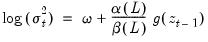 | (27.34) |
where
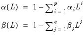 | (27.35) |
and
 | (27.36) |
For

, substituting

yields the EGARCH(1, 1) variance specification
 | (27.37) |
which may be compared with the corresponding EGARCH(1, 1) using the EViews (Equation 26.22) alternative specification
 | (27.38) |
The FIEGARCH model adds a long-run lag polynomial to
Equation (27.34)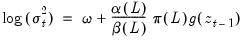 | (27.39) |
The corresponding FIEGARCH(1, 1) is given by
 | (27.40) |
Substituting using

yields
 | (27.41) |
As with the FIGARCH model, in practice the infinite sums are truncated at a finite number, typically 1,000 terms.
Estimating a FIEGARCH model
To estimate a FIEGARCH model in EViews simply select in the dropdown at the bottom of the dialog to display the GARCH dialog, then choose FIEGARCH in the section Model dropdown menu.
Note that since as EViews only supports the FIEGARCH(1, 1) specification, you may not specify the number of ARCH and GARCH terms.
You may, as for standard FIGARCH estimation, specify the Lag truncation number.
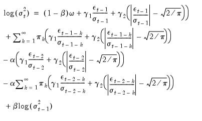
Mixed Data Sampling GARCH (MIDAS GARCH)
Mixed Data Sampling (MIDAS) regression is an estimation technique which allows for data sampled at different frequencies to be used in the same regression. For MIDAS GARCH models, the goal is to incorporate information from a large number of lags of a lower frequency series into an ARCH regression; incorporating, for example, lags of quarterly data in a monthly data GARCH model.
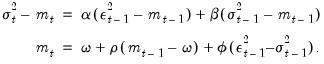
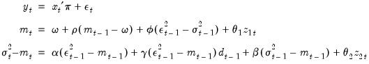
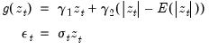
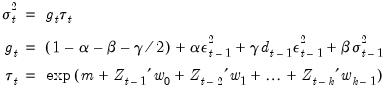
EViews 14 estimates the multiplicative component MIDAS GARCH(1,1) model of Conrad and Kleen (2020), where the mean equation is given by
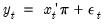 | (27.42) |
and the error variance

is the product of a transitory GARCH component

and a permanent component

,
 | (27.43) |
where

are explanatory variables,

is a dummy variable indicating negative shocks, and

are

lags of lower frequency exogenous variables.
Notably,
• the transitory component

is modeled as a GARCH(1, 1), with a restricted intercept term.
• the dummy variable

and associated coefficient

allow you to introduce asymmetry in the transitory component; if

the component is symmetric.
• the permanent component

is modeled using an intercept term

and

lags of

with weights

.
The underlying model is similar to the asymmetric Component GARCH(1,1) model
(27.27). Here, the transitory and permanent variance components are multiplicative instead of additive, and the permanent component is modeled using the lower frequency

variable lags.
Typically, researchers employ a full year of lags in modeling the permanent component so there may be a large number of

parameters to be estimated,
e.g.,

for a single monthly variable, and

for a single weekly variable.
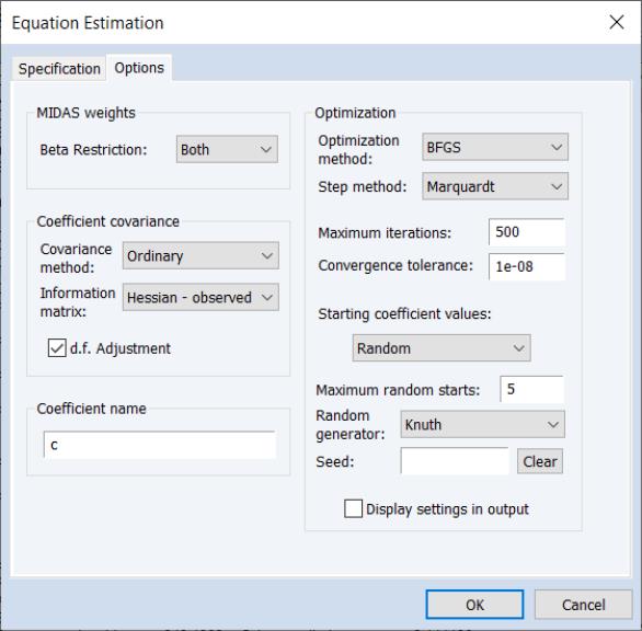
To reduce the number of parameters, we use a MIDAS weighting function to model the weights. Following Conrad and Kleen (2020), we employ a slightly modified version of the Ghysels, Santa-Clara and Valkanov (2004) beta function weighting scheme, where we parameterize the

in terms of a slope parameter

, and a small number of

weights:
The beta weighting function is extremely flexible and can take many shapes, including gradually increasing or decreasing, flat, humped, or U-shaped, depending on the values of the three MIDAS parameters

.
In practice, the parameters of the beta function are often further restricted by imposing a shape restriction (

), an endpoint restriction (

), or both restrictions (

and

) (see
“Beta Weighting” for related discussion).
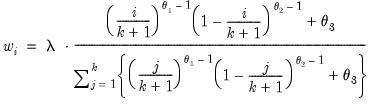
How to Estimate MIDAS GARCH in EViews
To estimate a MIDAS GARCH equation in EViews, the dated page with the high-frequency data must be active, and the lower-frequency data used to model the long-run component must be in a separate, low-frequency page.
Next, create an equation object by selecting or from the main menu, or enter the keyword equation in the command window. Select in the drop-down menu. Alternately, entering the keyword arch in the command window will create a new equation object and automatically set the main estimation method.
EViews will display the base ARCH dialog. Change the drop down menu in the middle of the page to to display the MIDAS GARCH page:
There are three distinct sections in the tab of the dialog.
• The section contains settings for the specification of the mean. Enter the specification by list, providing the name of the dependent variable followed by any mean regressors.
The drop down menu may be used to determine whether to add a variance term to the mean equation. You may choose between adding , , , or to the specification.
• The section contains settings for the variance equation.
The transitory variance for MIDAS models is a GARCH(1, 1). The checkbox may be used to include an asymmetric component in the transitory specification so that EViews will estimate
Equation (27.42) with

as a free parameter. If this option is not specified, EViews will enforce symmetry by setting

.
The permanent component for MIDAS uses lags of a low frequency regressor. You should enter the name of a single permanent component regressor in the Low frequency regressor edit field. Note that EViews only allows the specification of a single low frequency regressor. The syntax for specifying this variable is pagename\seriesname where pagename is the name of the page containing the series, and seriesname is the name of the series. You should use the Lag edit field to specify the number of low frequency regressor lags to include in the permanent component.
• The section contains the usual drop down for estimation method and the sample specification.
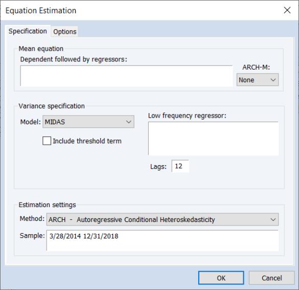
Clicking on the page shows a variety of MIDAS GARCH options:
• The section consists of a drop down where you may specify restrictions on the parameters of the MIDAS beta weighting function. You may use the menu to choose (no restrictions), (a shape restriction where

, (an endpoint restriction where

), or (both shape and endpoint restrictions). See
“Beta Weighting” for discussion.
• The section offers the standard choices coefficient covariance estimation methods.
• The edit field allows you to specify the name of a coefficient object to use in estimation.
• The section controls settings associated with estimation.
The top portion of the section offers the usual settings for estimating ARCH equations.
The drop-down allows you to choose between , (Gauss-Newton-OPG), , and the default optimization. The hybrid method is a combination of the and methods, where OPG is used for an initial 50 iterations, then BFGS is used until convergence. We have found that the hybrid method often reaches convergence more successfully than OPG or BFGS alone.
The menu allow you to choose the approach for choosing candidate iterative steps. The default method is , but you may instead select or .
The estimation process achieves convergence if the stopping rule is reached using the tolerance specified in the . Iterative estimation stops when the is reached, regardless of whether the convergence is achieved.
The remaining section controls starting values for the iterative estimation.
Baseline initial coefficient values are obtained by setting

,

,

(if relevant),

,

, and

, then performing OLS assuming those values to obtain starting values for

.
The drop down menu allows you to specify (the baseline starting values), fractions of the baseline values, , (using the contents of the default coefficient vector in the workfile), or the default entry, . The method first uses the baseline starting values, then if convergence is not achieved, chooses random values for the coefficients until convergence is achieved, or until the is reached. The

are drawn from a Uniform(0, 1) distribution and the

are drawn from a Uniform(-2, 2) distribution.
The randomization procedure is governed by the specified and the random fields. You may provide an integer value from 0 to 2,147,483,647, or you may the leave the field blank, in which case EViews will use the clock to obtain a seed at the time of estimation.
Working with MIDAS GARCH Equations
Almost all of the views and procedures for a standard GARCH model work identically for a MIDAS GARCH equation. We offer brief comments on a couple of views.
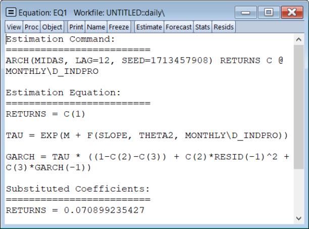
Representations
The view () offers text representations of the estimation command string, and the mean and variance equations.
The mean equation shows that RETURNS is simply equal to the intercept. The GARCH variance equation shows the multiplicative form of the equation using both the underlying coefficients and substituted values.
In contrast to most EViews Representations views, however, the MIDAS GARCH Representations view does not provide expressions that may be evaluated using the EViews. Notably, the equation for TAU is only a pseudo-representation of the permanent component specification. Thus, the TAU and GARCH equations may not be evaluated without additional modification.
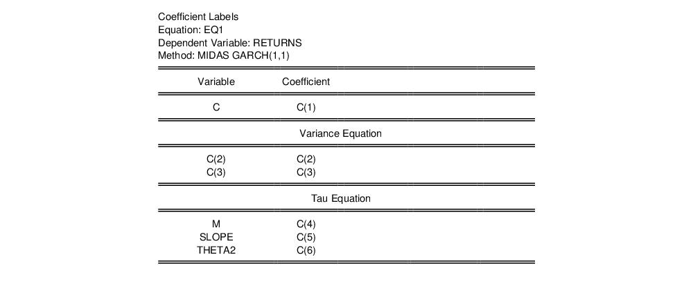
Coefficient Labels
The coefficient label view makes it easy to map the results in the main estimation output to the underlying coefficient values. This is especially useful in allowing you to see the coefficients corresponding to the different variance components.
To see the coefficient label view, click on :
The view makes it easy to see that the long-run components for the estimator are C(4), C(5) and C(6).
User Specified Models
In some cases, you might wish to estimate an ARCH model not mentioned above, for example a special variant of PARCH. Many other ARCH models can be estimated using the logl object. For example,
“The Log Likelihood (LogL) Object” contains examples of using logl objects for simple bivariate GARCH models.