Background
Standard regression models require the regressor data to follow the same frequency and structure as the dependent variable in the regression. This restriction is not always met in practice—as in economics, where major statistical releases occur on annual, quarterly, monthly and even daily frequencies.
Traditionally, there have been two approaches to estimation in mixed frequency data settings:
• The first approach involves introducing the sum or average of the higher frequency data into the lower frequency regression. This approach adds a single coefficient for each high frequency variable, implicitly applying equal weighting to each value in the sum.
• Alternately, the individual components of the higher frequency data may be added to the regression, allowing for a separate coefficient for each high frequency component. For example, in estimating an annual regression with monthly high frequency regressors, one could add each of the monthly components as a regressor. Note that this approach adds a large number of coefficients to the regression.
MIDAS estimation occupies the middle ground between these approaches, allowing for non-equal weights but reducing the number of coefficients by fitting functions to the parameters of the higher frequency data. Thus, MIDAS offers an approach to mixed frequency estimation featuring a flexible, parsimonious parameterization of the response of the lower frequency dependent variable to the higher frequency data.
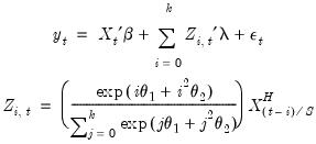
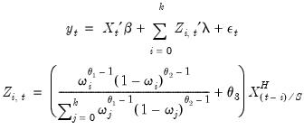
Specifically, the model under consideration is:
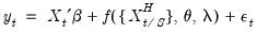 | (30.1) |
where
• 
is the dependent variable, sampled at a low frequency, at date

,
• 
is the set of regressors sampled at the same low frequency as

,
• 
is a set of regressors sampled at a higher frequency with

values for each low frequency value. Note that

is not restricted to the

values associated with the current

as it may include values corresponding to lagged low frequency values.
• 
is a function describing the effect of the higher frequency data in the lower frequency regression
• 
,

, and

vectors of parameters to be estimated.
The individual coefficients approach adds each of the higher frequency components as a regressor in the lower frequency regression. In the simple case where we only include high frequency data corresponding to the current low frequency observation, we have:
 | (30.2) |
where

are the data

high frequency periods prior to

(we will refer to these data as the

-th high frequency lag at

). Notice that this approach estimates a distinct

for each of the

high frequency lag regressors.
Alternately, the simple aggregation approach adds an equally weighted sum (or average) of the high frequency data as a regressor in the low frequency regression:
 | (30.3) |
The approach estimates a single

associated with the new regressor. Viewed differently, the aggregation approach may be thought of as one in which the component higher frequency lags all enter the low frequency regression with a common coefficient

.
For a quarterly regression with a higher frequency monthly series, there are three months in each quarter so the individual coefficients approach adds three regressors to the low frequency regression. The first regressor contains values for the first month in the corresponding quarter (January, April, July, or October), the second regressor has values for the second month in the corresponding quarter (February, May, August, or November), and the third regressor contains values for the third month in the relevant quarter (March, June, September, December).
The aggregation approach adds the single regressor containing the sum of the monthly values over the corresponding quarter. For first quarter observations, the regressor will contain the sum of the higher frequency January, February, and March monthly values for that quarter. Similarly, the regressor will contain the sum of the October, November, and December values in fourth quarter observations.
We may think of these two approaches as polar extremes. The individual coefficients approach offers the greatest flexibility but requires large numbers of coefficients. The aggregation approach is parsimonious, but places quite significant equal weighting restrictions on the lagged high frequency data.
In contrast, MIDAS estimation offers several different weighting functions which occupy the middle ground between the unrestricted and the equally weighted aggregation approaches. The MIDAS weighting functions reduce the number of parameters in the model by placing restrictions on the effects of high frequency variables at various lags.
Step Weighting
The simplest weighting method employs the step function:
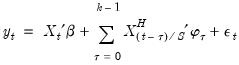 | (30.4) |
where
• 
is a chosen number of lagged high frequency periods to use (where

may be less than or greater than

).
• 
is a step length
• 
for
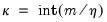
In this approach, the coefficients on the high frequency data are restricted using a step function, with high frequency lags within a given step sharing values for

. For example, with

, the first three lagged high frequency lags

,

, employ the same coefficient

, the next three lags use

, and so on up to the maximum lag of

.
Notably, the number of high frequency coefficients in the step weighting model increases with the number of high frequency lags, but in comparison to an individual coefficient approach, the number of coefficients is reduced by a factor of roughly

.
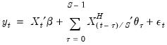
Almon (PDL) Weighting
Almon lag weighting (also called polynomial distributed lag or PDL weighting) is widely used to place restrictions on lag coefficients in autoregressive models, and is a natural candidate for the mixed frequency weighting.
For each high frequency lag up to

, the regression coefficients are modeled as a

dimensional lag polynomial in the MIDAS parameters

. We may write the resulting restricted regression model as:
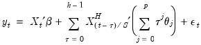 | (30.5) |
where

is the Almon polynomial order, and the chosen number of lags

may be less than or greater than

.
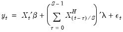
Importantly, the number of coefficients to be estimated depends on the polynomial order and not the number of high frequency lags. We can see this more clearly after rearranging terms and rewriting the model using a constructed variable:
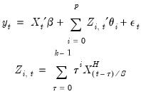 | (30.6) |
It is easy to see the distinct coefficient

associated with each of the

sets of constructed variables

.
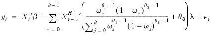
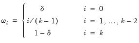
Exponential Almon Weighting
The normalized exponential Almon weighting approach uses exponential weights and a lag polynomial of degree 2, yielding:
 | (30.7) |
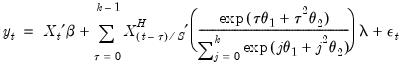 | (30.8) |
where

is a chosen number of lags,

is a slope coefficient that is common across lags, and the differential response comes via the exponential weighting function and the lag polynomial which depends on the two MIDAS coefficients

and

.
In constructed variable form, we have
 | (30.9) |
Note that this regression model is highly nonlinear in the parameters of the model.
Beta Weighting
Beta weighting was introduced by Ghysels, Santa-Clara and Valkanov (2004) and is based on the normalized beta weighting function. The corresponding regression model is given by
 | (30.10) |
where

is a number of lags,

is a slope coefficient that is common across lags, and
 | (30.11) |
where

is a small number (in practice, approximately equal to

).
In constructed variable form, we have
 | (30.12) |
The beta function is extremely flexible and can take many shapes, including gradually increasing or decreasing, flat, humped, or U-shaped, depending on the values of the three MIDAS parameters

.
In practice the parameters of the beta function are restricted further by imposing

,

, or

and

.
• The restriction

implies that the
shape of the weight function depends on a single parameter, exhibiting slow decay when

and slow increase when

.
• The restriction

implies that there are zero weights at the high frequency lag endpoints (when

and

).
• The restriction

and

imposes both the shape and the zero endpoint weight restrictions.
(Please note that for specifications with a small number of MIDAS lags the zero endpoint restriction is quite restrictive and may generate significant bias.)
Lastly, while the number of parameters of the beta weighting model is at most 3 and does not increase with the number of lags, estimation does involve optimization of a highly non-linear objective.
U-MIDAS
The U-MIDAS technique adds each of the higher frequency components as a regressor in the lower frequency regression. Notably, The U-MIDAS weighting method is simply the individual coefficients technique given by
Equation (30.2). In contrast to other methods, there are no restrictions on the implied lag polynomial in the low frequency regression.
While extremely flexible, U-MIDAS requires a estimation of a large number of coefficients. U-MIDAS does not alleviate the issue of requiring a large number of coefficients, but can be used in cases where a small number of lags are required, and is often used for comparative purposes.
Auto/GETS
The Auto/GETS weighting scheme is an extension of U-MIDAS that uses variable selection to reduce down the number of individual coefficients by excluding individual lags. See
“Auto-Search / GETS” for discussion of the Auto/GETS procedure.
As a complement to the MIDAS variable selection, EViews also offers the ability to test for indicator variable inclusion. See
“Indicator Saturation” for additional detail on indicator saturation.