Background
While the ordinary least squares estimator (OLS) is notably unbiased, it can exhibit large variance. If, for example, the data have more regressors

than the length of the dataset

(sometimes referred to as the “large

, small

problem”) or there is high correlation between the

regressors, least squares estimates are very sensitive to random errors, and suffer from over-fitting and numeric instability.
In these and other settings, it may be advantageous to perform regularization by specifying constraints on the flexibility of the OLS estimator, resulting in a simpler or more parsimonious model. By restricting the ability of the ordinary least squares estimator to respond to data, we reduce the sensitivity of our estimates to random errors, lowering the overall variability at the expense of added bias. Thus, regularization trades variance reduction for bias with the goal of obtaining a more desirable mean-square error.
One popular approach to regularization is elastic net penalized regression.
Elastic Net Regression
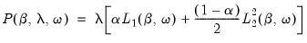
In estimating elastic net penalized regression for regularization, the conventional sum-of-squared residuals (SSR) objective is augmented by a penalty that depends on the absolute and squared magnitudes of the coefficients. These coefficient penalties act to shrink the coefficients magnitudes toward zero, trading off increases in the sums-of-squares against reductions in the penalties.
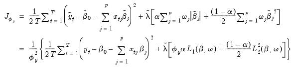
We may write the elastic net cost or objective function as,
 | (37.1) |
for a sample of

observations on the dependent variable and

regressors:

,

:
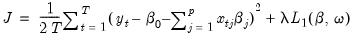
• The first term in this expression,
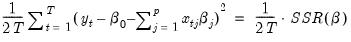 | (37.2) |
is the familiar sum-of-squared residuals (SSR), divided by two times the number of observations.
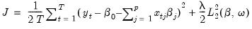
• The second term is the penalty portion of the objective,
 | (37.3) |
for

, and where the

norm is the

‑weighted sum (

) of the absolute values of the coefficient values,
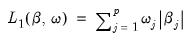 | (37.4) |
and the squared

norm is the

‑weighted sum of the squared values of the coefficient values,
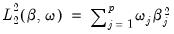 | (37.5) |
Typically, the coefficients are penalized equally so that

for all

.
In general, the problem of minimizing this objective with respect to the coefficients

does not have a closed-form solution and requires iterative methods, but efficient algorithms are available for solving this problem (Hastie, Friedman, and Tibshirani 2010).
The Penalty Parameter
Elastic net specifications rely centrally on the penalty parameter

, (

), which controls the magnitude of the overall coefficient penalties. Clearly, larger values of

are associated with a stronger coefficient penalty, and smaller values with a weaker penalty. When

, the objective reduces to that of standard least squares.
One can compute Enet estimates for a single, specific penalty value, but the recommended approach (Hastie, Friedman, and Tibshirani, 2010) is to compute estimates for each element of a set of values and to examine the behavior of the results as

varies from high to low.
When estimates are obtained for multiple penalty values, we may use model selection techniques to choose a “best”

.
Automatic Lambda Grid
Researchers will usually benefit from practical guidance in specifying

values.
Friedman, Hastie, and Tibshirani (2010) describe a recipe for obtaining a path of penalty values:
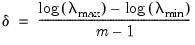
• First, specify a (maximum) number of penalty values to consider, say

.
• Next employ the data to compute the smallest

for which all of the estimated coefficients are 0. The resulting

will be the largest value of

to be considered.
For ridge regression specifications, coefficients are not easily pushed to zero, so we arbitrarily use an elastic net model with

to determine

.
• Specify

, the smallest value of

to be considered, as a predetermined fractional value of

.
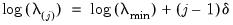
• Compute a grid of

descending penalty values on a natural log scale from

to

so that
for

, where
• Take exponents of the values, yielding the lambda path
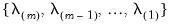
.
Path Estimation
Friedman, Hastie, and Tibshirani (2010) describe a path estimation procedure in which one estimates models beginning with the largest value

and starting coefficient values of 0, and continuing sequentially from

to

or until triggering a stopping rule. The procedure employs what the authors term “warm starts” with coefficients obtained from estimating the

model used as starting values for estimating the

model.
Bear in mind that while

is derived so that the coefficients values are all 0, an arbitrarily specified fractional value

has no general interpretation. Further, estimation at a given

for

can be numerically taxing, might not converge, or may offer negligible additional value over prior estimates. To account for these possibilities, we may specify rules to truncate the

-path of estimated models when encountering non-convergent or redundant results.
Friedman, Hastie, and Tibshirani (2010) propose terminating path estimation if the sequential changes in model fit or changes in coefficient values cross specific thresholds. We may, for example, choose to end path estimation at a given

if the

exceeds some threshold, or the relative change in the SSR falls below some value. Similarly, if model parsimony is a priority, we might end estimation at a given

if the number of non-zero coefficients exceeds a specific value or a specified fraction of the sample size.
Model Selection
We may use cross-validation model selection techniques to identify a preferred value of

from the complete path. Cross-validation involves partitioning the data into training and test sets, estimating over the entire

path using the training set, and using the coefficients and the test set to compute evaluation statistics.
There are a number of different ways to perform cross-validation. See
“Cross-validation Settings” and
“Cross-validation Options” for discussion and additional detail.
If a cross-validation method defines only a single training and test set for a given

, the penalty parameter associated with the best evaluation statistic is selected as

.
If the cross-validation method produces multiple training and test sets for each

, we average the statistics across the multiple sets, and the penalty parameter for the model with the best average value is selected as

. Further, we may compute the standard error of the mean of the cross-validation evaluation statistics, and determine the penalty values

and

corresponding to the most penalized models with average values within one and two standard errors of the optimum.
The Penalty Function
Note that the penalty function
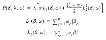 | (37.6) |
is comprised of several components: the overall penalty parameter

, the coefficient penalty terms

and

, individual penalty weights

, and the mixing parameter

.
There are many detailed discussions of the varying properties of these penalty approaches (see, for example Friedman, Hastie, and Tibshirani (2010).
For our purposes it suffices to note that

term is quadratic with respect to the representative coefficient

. The derivatives of the

norm
are of the form

, so that the absolute value of the
j-th derivative increases and decreases with the weighted values of

. Crucially, the derivative approaches 0 as

approaches 0.
In contrast,

is linear in the representative coefficient

, with a constant derivative of

for all values of

.
The Mixing Parameter
The

mixing parameter controls the relative importance of the

and

penalties in the overall objective. Larger values of

assign more importance to

while smaller values assign more importance to

.
There are many discussions of the properties of the various penalty mixes. See, for example Hastie, Tibshirani, and Friedman (2010) for discussion of the implications of different choices for

.
For our purposes, we note only that models with penalties that emphasize the

norm component tend to have more zero coefficients than models which feature the

penalty, as the derivatives of the

remain constant as the coefficient approaches zero, while the derivatives of the

norm for a given coefficient become negligible in the neighborhood of zero.
The limiting cases for the mixing parameter,

, and

are themselves well-known estimators.
Setting

yields a
Lasso (Least-Absolute Shrinkage and Selection Operator) model that contains only the

-norm penalty:
 | (37.7) |
Setting

produces a
ridge regression specification with only the

-penalty:
 | (37.8) |
The ridge regression estimator for this objective has an analytic solution. Writing the objective in matrix form:
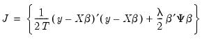 | (37.9) |
for
where

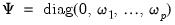
corresponds to the unpenalized intercept. Differentiating the objective yields:
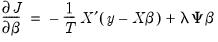 | (37.10) |
Setting equal to zero and collecting terms
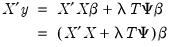 | (37.11) |
so that a analytic closed-form estimator exists,
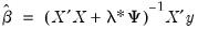 | (37.12) |
which is recognizable as the traditional ridge regression estimator with ridge parameter

and diagonal adjustment weights

, where

.
Thus, while an elastic net model with

is a form of ridge regression, it is important to recognize that the parameterization of the diagonal adjustment differs between elastic net ridge and traditional ridge regression, with the former using

and the latter using

.
Bear in mind that in EViews, the coefficient on the intercept term “C” is not penalized in either ridge or in elastic net specifications. Comparison to results obtained elsewhere should ensure that intercept coefficient penalties are specified comparably.
Individual Penalty Weights
The notation in
Equation (37.1) explicitly accounts for the fact that we do not wish to penalize the

intercept coefficient.
We may generalize this type of coefficient exclusion using individual penalty weights

for

to attenuate or accentuate the impact of the overall penalty

on individual coefficients.
Notably, setting

for any

implies that

is not penalized. We may, for example, express the intercept excluding penalty in
Equation (37.1) using

and

terms that sum over all

coefficients (including the intercept) with

:
 | (37.13) |
where

is a composite individual penalty weight associated with coefficient

.
For comparability with the baseline case where the weights are 1 for all but the intercept, we normalize the weights so that

where

is the number of non-zero

.
Data scaling
Scaling of the dependent variable and regressors is sometimes carried out to improve the numeric stability of ordinary least squares regression estimates. It is well-known that scaling the dependent variable or regressors prior to estimation does not have substantive effects on the OLS estimates:
• Dividing the dependent variable by

prior to OLS produces coefficients that equal the unscaled estimates divided by

and an SSR equal to the unscaled SSR divided by

.
• Dividing each of the regressors by an individual scale

prior to OLS produces coefficients equal to the unscaled estimates multiplied by

. The optimal SSR is unchanged.
Following estimation, the results may easily be returned to the original scale:
• The effect of dependent variable scaling is undone by multiplying the estimated scaled coefficients by

and multiplying the scaled SSR by

.
• The effect of regressor scaling is undone by dividing the estimated coefficients by the

.
These simple equivalences do not hold in a penalized setting. You should pay close attention to the effect of your scaling choices, especially when comparing results across approaches.
Dependent Variable Scaling
In some settings, scaling the dependent variable only changes the scale of the estimated coefficients, while in others, it will change both the scale and the relative magnitudes of the estimates.
To understand the effects of dependent variable scaling, define the objective function using the scaled dependent variable,

and corresponding coefficients

and penalty

. We will see whether imposing the restricted parametrization,

alters the objective function.
We may write the restricted objective as:
where

is the penalty associated with the scaled data objective. Notice that this objective using scaled coefficients is not, in general, a simple scaled version of the objective in
Equation (37.1) since the

term is scaled by an additional

and the

is not.
Inspection of this objective yields three results of note:
• If

, the relative importance of the residual and the penalty portions of the objective are unchanged from
Equation (37.1) if

. Thus, the estimates for Lasso model coefficients using the scaled dependent variable will be scaled versions of the unscaled data coefficients obtained using an appropriately scaled penalty.
• If

, then the relative importance of the residual and the penalty portions of the objective is unchanged for

. Thus, for elastic net ridge regression models, the scaling of the dependent variable produces an equivalent model at the same penalty values.
• For

, it is not possible to find a

where the simple scaling of coefficients does not alter the relative importance of the residual and penalty components, so estimation of the scaled dependent variable model results in coefficients that differ by more than scale.
Regressor Scaling
The practice of standardizing the regressors prior to estimation is common in elastic net estimation.
As before, we can see the effect by looking at the effect of scaling on the objective function. We define a new objective using the scaled regressors

and coefficients

,

, and corresponding penalty

, and impose the restriction that the new coefficients are individual scaled versions of the original coefficients,

.
We have:
 | (37.14) |
Since coefficients in the penalty portion are individually scaled while those in the SSR residual portion are not, there is no general way to write this objective as a scaled version of the original objective. The coefficient

estimates will differ from the unweighted estimates by more than just individual variable scale.
Summary
To summarize, when comparing results between different choices for scaling, you should remember that results may differ substantively depending on your choices:
• Scaling the dependent variable (

) produces ridge regression coefficients that are simple

scaled versions of those obtained using unscaled data. For Lasso regression, a similar scaled coefficient result holds provided the penalty parameter is also scaled accordingly.
• Scaling the dependent variable (

) prior to

elastic net estimation produces scaled and unscaled coefficient estimates that differ by more than scale.
• Scaling the regressors (

) prior to estimation produces coefficient results that differ by more than the individual scales from those obtained using unscaled regressors.