Working with Elastic Net Equations
An elastic net equation estimated by EViews is a penalized regression specification featuring a number of specialized views and procedures. We describe below the basics of working with your estimated equation
Estimation Output
After you estimate your elastic net specification, EViews will display the main estimation output table which is customized for penalized regression. Alternatively, you can display the output by clicking on .
If you specify a single penalty parameter, EViews will display a single column of results:
Note that estimation at a single penalty value as illustrated here is not recommended by Hastie, Tibshirani, and Friedman (2010). For a variety of reasons, they recommend estimating models for an entire

-path.
The header portion of the output describes the underlying equation specification information, including the sample information, the penalty specification, the specified penalty parameter, and any scaling of dependent variable or regressor scaling.
Here, we have estimated an elastic net model with

and user-specified

. There was no dependent variable scaling and the regressors were scaled using the population standard deviation.
The next section of the output shows the non-zero estimated coefficients reported at the original data scale. Notably, AGE, LBPH, and the other variables with zero coefficient are omitted. Note that standard errors are not provided for the penalized regression estimators since they may be misleading given the inherently biased nature of the estimator.
Below the coefficients section are reports of the usual measures of fit (, , , ), along with information on the number of and . In this case, in addition to the 3 displayed non-zero coefficients, there are 6 coefficients that estimation set to zero.
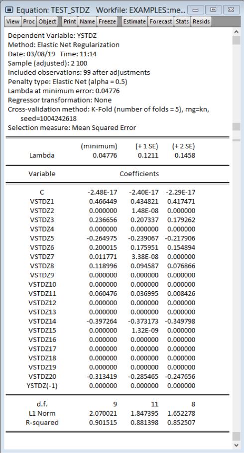
If you specify more than one penalty parameter, EViews will display modified output:
In addition to basic information, the header section now describes the path used in estimation. Here we see that the
values are automatically determined, that the optimal
of 0.11228 is selected using K-Fold cross-validation using a mean-squared error objective function and 5 folds.
If 3 or more penalties are provided, the coefficient output will have 3 columns of output. The first column shows estimation results for the optimal
. The remaining columns illustrate the trade-off between higher penalties and poorer values of the cross-validation selection objective by displaying results for the most penalized specifications with objective values within 1 and 2 standard deviations of the optimum.
Here, 0.367659 is the largest
yielding a cross-validation MSE within 1 standard deviation of the optimum, and 0.521147 is the largest
producing a cross-validation MSE within 2 standard deviations of the optimum.
For 3 or fewer penalties, the output will display a column for each penalty value.
The coefficients section of the output shows estimates for
all coefficients which are non-zero for at least one of the displayed penalty values. The coefficients for LBPH and PGG45, for example, are non-zero at the optimal
value, but are 0 for the two other higher penalized specifications. Similarly the estimated coefficient for LWEIGHT is non-zero for the two lower
values, but is 0 for the larger penalty.
The summary section at the bottom of the table shows the measures of fit, and information about the number of zero and non-zero coefficients for each value of
.
The columns in this table may show results for only a subset of the

in the path. Additional information about the full set of path coefficients, measures of fit, and cross-validation information is available in other equation views.
Elastic Net Views and Procs
While many of the views and procs for other equation estimators are not applicable in elastic net equations, most of those that are supported are based on the results for the optimal

, but are otherwise self-explanatory. For example, the and views simply shows the standard views using residuals computed using results for the optimal

. Similarly, the proc produces forecasts using coefficients obtained using the sole or optimal

.
We focus here on the views specific to elastic net estimators. The views are divided into three main categories: coefficient path, lambda path, and model selection.
Coefficient Path
The views show the behavior of the coefficient estimates along the

-path. The results are displayed in graphical or matrix table form:
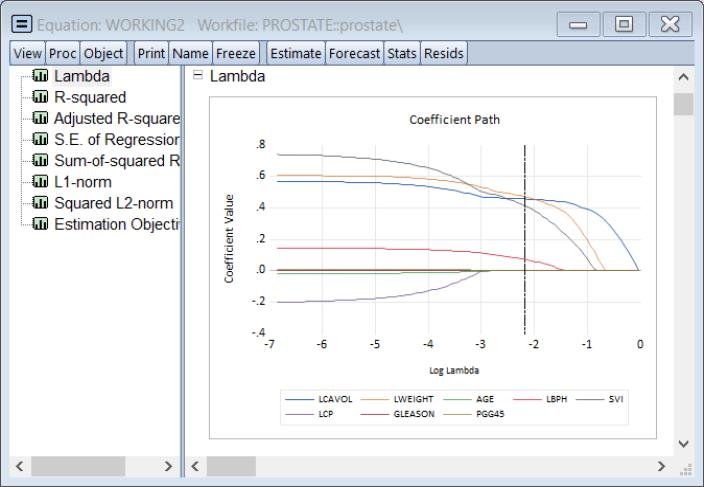
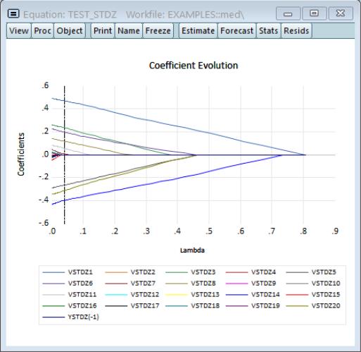
Graphs
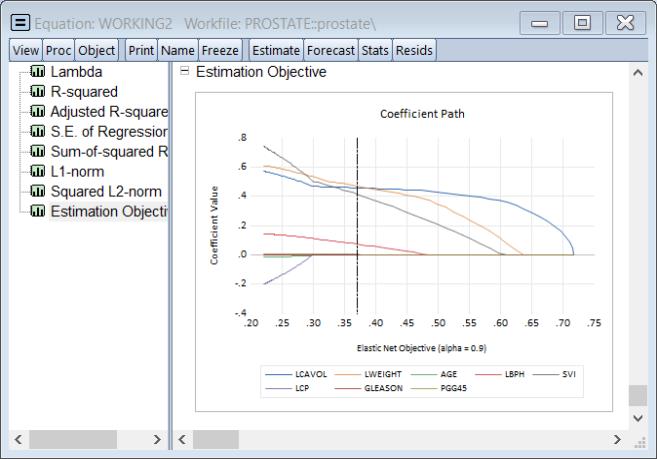
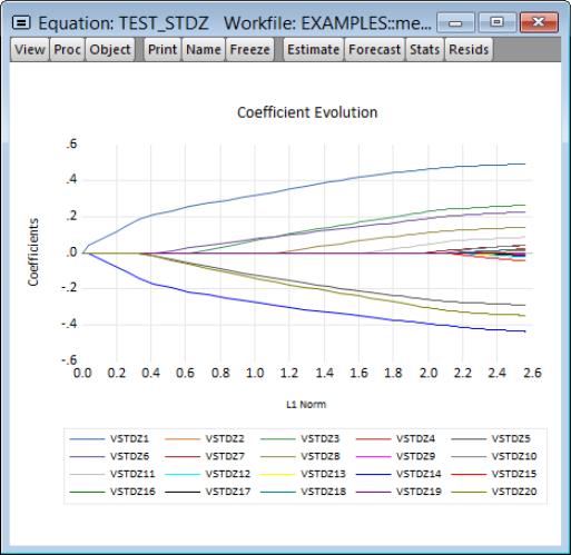
If you select EViews displays a spool containing graphs of coefficient values against various values defined along the

-path:
The graph is a plot of each of the coefficients (excluding the intercept) against the log of the penalty parameter showing the effect of increasing the penalty parameter on the estimates; as the value of the regularization penalty increases, the absolute value of each of the coefficients decreases, with coefficient driven to zero for large enough penalties.
Note that EViews will only display non-intercept coefficients that have a non-zero value in the path; coefficients that are always zero are not displayed and the graph titles will be modified to reflect this fact.
The vertical line shows the value of the log lambda at the cross-validation optimum.
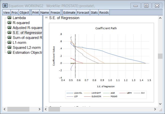
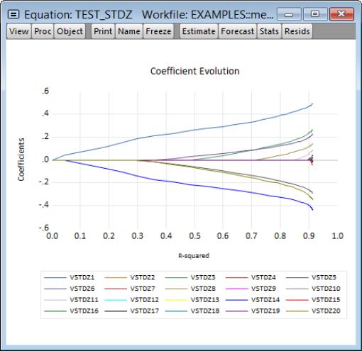
The next set of graphs plot coefficients against various measures of fit such as the , , and :
The remaining graphs plot the non-intercept coefficients against the components of the estimation objective function: the , the of the coefficients, the of the coefficients, and the :
All of these graphs display a vertical line at the value corresponding to the cross-validation optimum

.
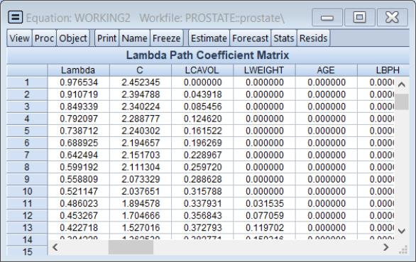
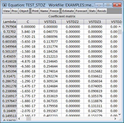
Lambda Path Matrix
To display the coefficient values for the entire path of

values, select .
The sheet shows the values of the coefficients along with the corresponding values of

. If there are coefficients that have only zero values along the path, they will be dropped and the title will change to reflect this fact.
Lambda Path
The views show the behavior of various log values along the

-path. The results are displayed in graphical or table form:
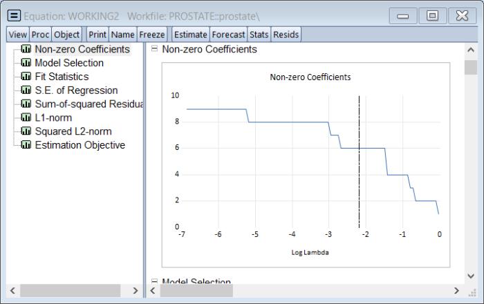
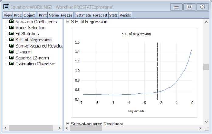
Graphs
If you select , EViews displays a spool containing graphs of various values against the log

values in the path:
All of the graphs display results plotted against the corresponding values of the log

in the path:
• The graph plots the number of non-zero coefficients.
• The graph plots the model selection objective.
• The graph plots the

and Adjusted

.
• The , , , and display the corresponding elements of the estimation objective function.
The vertical line shows the value of the log of lambda at the cross-validation optimum.
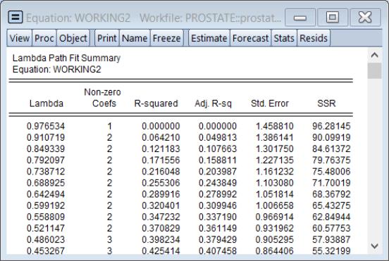
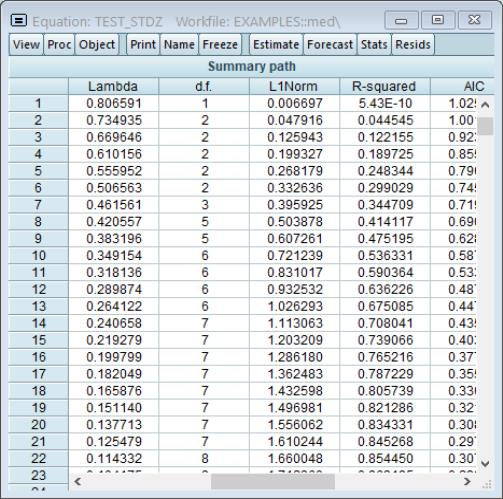
Fit Summary
Selecting displays a table showing the number of non-zero coefficients, the

and adjusted

fit statistics, and the SSR for the

values in the path:
The row containing the selected optimal penalty will be highlighted.
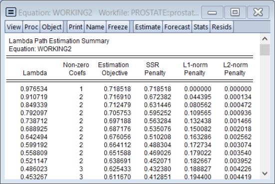
Estimation Summary
Selecting displays a table showing the number of non-zero coefficients, estimation objective, components of the estimation objective, and the convergence status of the estimates for each

value in the path:
The , , and are the individual components of the in
Equation (37.1).
The row containing the selected optimal penalty will be highlighted.
Model Selection
The views summarize results from the model selection procedure used to determine the optimal value of

. While some of these views are standard model selection views, others have been customized for the current setting.
Criteria Graph
Click on to show the top values for the model selection criteria along the corresponding

:
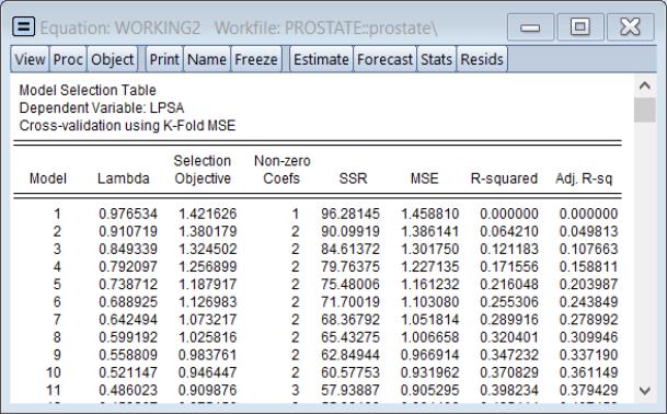
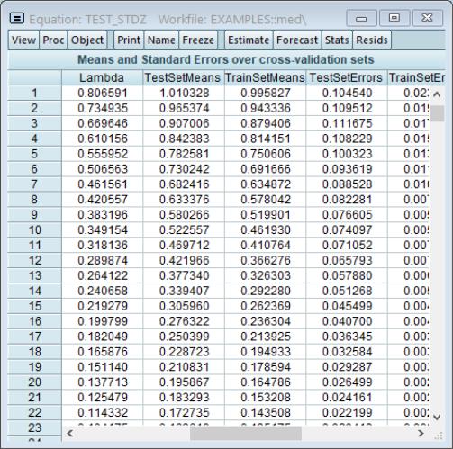
Summary Table
Selecting to show a table of model selection and fit statistics:
The column shows the values of the objective, in this case the K-Fold MSE, for each value of

. Also displayed are the number of associated with this specification.
The columns for , , , are measures of fit for the models associated with

. They repeat the information from the to provide additional context to the model selection results.
The row containing the selected optimal penalty will be highlighted.
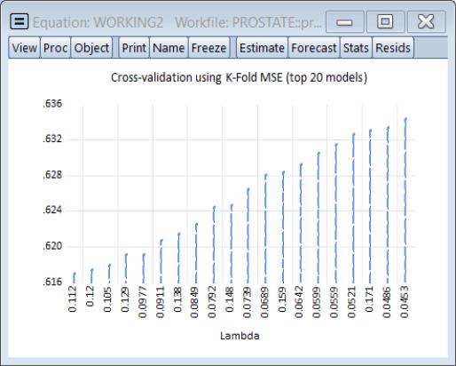
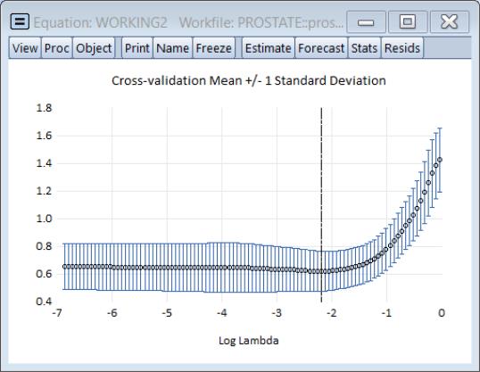
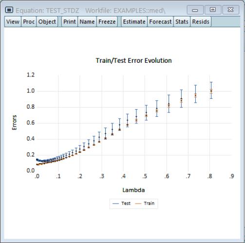
Cross-validation Graph
The cross-validation error graph (), offers additional information about the distribution of the cross-validation results, showing the mean and +/- 1 standard deviation of the objective for each value of log

.
The vertical line shows the value of the log of the penalty parameter at the cross-validation optimum.
Forecast
Clicking on brings up the standard forecast dialog. EViews will produce a forecast using the coefficients associated with the optimal penalty parameter if estimates are available for more than one

.