Factor Views
EViews provides a number of factor object views that allow you to examine the properties of your estimated factor model.
Specification
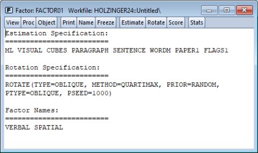
The specification view provides a text representation of the estimation specification, as well as the rotation specifications and assigned factor names (if relevant).
In this example, we see that we have estimated a ML factor model for seven variables, using a convergence criterion of 1e-07. The model was estimated using the default SMCs initial communalities and Velicer’s MAP criterion to select the number of factors.
In addition, the object has a valid rotation method, oblique Quartimax, that was estimated using the default 25 random oblique rotations. If no rotations had been performed, the rotation specification would have read “Factor does not have a valid rotation.”
Lastly, we see that we have provided two factor names, “Verbal”, and “Spatial”, that will be used in place of the default names of the first two factors “F1” and “F2”.
Estimation Output
Select to display the main estimation output (unrotated loadings, communalities, uniquenesses, variance accounted for by factors, selected goodness-of-fit statistics). Alternately, you may click on the toolbar button to display this view.
Rotation Results
Click to show the output table produced when performing a rotation (rotated loadings, factor correlation, factor rotation matrix, loading rotation matrix, and rotation objective function values).
Goodness-of-fit Summary
Select to display a table of goodness-of-fit statistics. For models estimated by ML or GLS, EViews computes a large number of absolute and relative fit measures. For details on these measures, see
“Model Evaluation”.
Matrix Views
You may display spreadsheet views of various matrices of interest. These matrix views are divided into four groups: matrices based on the observed dispersion matrix, matrices based on the reduced matrix, fitted matrices, and residual matrices.
Observed Covariances
You may examine the observed matrices by selecting and the desired sub-matrix:
• The entry displays the original dispersion matrix, while the scales the original matrix to have unit diagonals. In the case where the original matrix is a correlation, these two matrices will obviously be the same.
• displays a matrix of the number of observations used in each pairwise comparison.
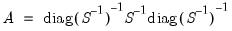
• If you select , EViews will display the anti-image covariance of the original matrix. The anti-image covariance is computed by scaling the rows and columns of the inverse (or generalized inverse) of the original matrix by the inverse of its diagonals:
• will display the matrix of partial correlations, where every element represents the partial correlation of the variables conditional on the remaining variables. The partial correlations may be computed by scaling the anti-image covariance to unit diagonals and then performing a sign adjustment.
Reduced Covariance
You may display the initial or final reduced matrices by selecting and or .
Fitted Covariances
To display the fitted covariance matrices, select and the desired sub-matrix. displays the estimated covariance using both the common and unique variance estimates, while displays the estimate of the variance based solely on the common factors.
Residual Covariances
The different residual matrices are based on the total and the common covariance matrix. Select and the desired matrix, , or . The residual matrix computed using the total covariance will generally have numbers close to zero on the main diagonal; the matrix computed using the common covariance will have numbers close to the uniquenesses on the diagonal (see
“Scaling” for caveats).
Factor Structure Matrix
The factor structure matrix reports the correlations between the variables and factors. The correlation is equal to the (possibly rotated) loadings matrix times the factor correlation matrix,

; for orthogonal factors, the structure matrix simplifies so that the correlation is given by the loadings matrix,

.
Factor Selection
If you estimated your factor model using the Bai and Ng or the Ahn and Horenstein number of factor selection method, you may use this view to display information related to the selection procedure.
Loadings Views
You may examine your rotated or unrotated loadings in spreadsheet or graphical form.
You may to display the current loadings matrix in spreadsheet form. If a rotation has been performed, then this view will show the rotated loadings, otherwise it will display the unrotated loadings. To view the unrotated loadings, you may always select .
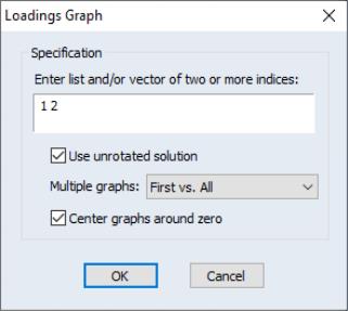
To display the loadings as a graph, select The dialog will prompt you for a set of indices for the factors you wish to plot. EViews will produce pairwise plots of the factors, with the loadings displayed as lines from the origin to the points labeled with the variable name.
By default, EViews will use the rotated solution if available; to override this choice, click on the checkbox.
The other settings allow you to control the handling of multiple graphs, and whether the graphs should be centered around the origin.
Scores
Select to compute estimates of factor score coefficients and to compute factor score values for observations. This view and the corresponding procedure are described in detail in
“Estimating Scores”.
Eigenvalues
One important class of factor model diagnostics is an examination of eigenvalues of the unreduced and the reduced matrices. In addition to being of independent interest, these eigenvalues are central to various methods for selecting the number of factors.
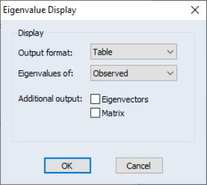
Select to open the dialog. By default, EViews will display a table view containing a description of the eigenvalues of the observed dispersion matrix.
The dialog options allow you to control the output format and method of calculation:
• You may change the to display a graph of the ordered eigenvalues. By default, EViews will display the resulting Scree plot along with a line representing the mean eigenvalue.
• To base calculations on the scaled observed, initial reduced or final reduced matrix, select the appropriate item in the dropdown.
• For table display, you may include the corresponding eigenvectors and dispersion matrix in the output by clicking on the appropriate checkbox.
• For graph display, you may also display the eigenvalue differences, and the cumulative proportion of variance represented by each eigenvalue. The difference graphs also display the mean value of the difference; the cumulative proportion graph shows a reference line with slope equal to the mean eigenvalue.
Additional Views
Additional views allow you to examine:
• The matrix of maximum absolute correlations ().
• The squared multiple correlations (SMCs) and the related anti-image covariance matrix ().
• The Kaiser-Meyer-Olkin (Kaiser 1970; Kaiser and Rice, 1974; Dziuban and Shirkey, 1974), measure of sampling adequacy (MSA) and corresponding matrix of partial correlations ().
The first two views correspond to the calculations used in forming initial communality estimates (see
“Communality Estimation”). The latter view is an “index of factorial simplicity” that lies between 0 and 1 and indicates the degree to which the data are suitable for common factor analysis. Values for the MSA above 0.90 are deemed “marvelous”; values in the 0.80s are “meritorious”; values in the 0.70s are “middling”; values the 60s are “mediocre”, values in the 0.50s are “miserable”, and all others are “unacceptable” (Kaiser and Rice, 1974).