Limited Information Maximum Likelihood and K-Class Estimation
Limited Information Maximum Likelihood (LIML) is a form of instrumental variable estimation that is quite similar to TSLS. As with TSLS, LIML uses instruments to rectify the problem where one or more of the right hand side variables in the regression are correlated with residuals.
LIML was first introduced by Anderson and Rubin (1949), prior to the introduction of two-stage least squares. However traditionally TSLS has been favored by researchers over LIML as a method of instrumental variable estimation. If the equation is exactly identified, LIML and TSLS will be numerically identical. Recent studies (for example, Hahn and Inoue 2002) have, however, found that LIML performs better than TSLS in situations where there are many “weak” instruments.
The linear LIML estimator minimizes
 | (23.16) |
with respect to

, where y is the dependent variable, X are explanatory variables, and Z are instrumental variables.
Computationally, it is often easier to write this minimization problem in a slightly differentform. Let

and

. Then the linear LIML objective function can be written as:
 | (23.17) |
Let

be the smallest eigenvalue of

. The LIML estimator of

is the eigenvector corresponding to

, with a normalization so that the first element of the eigenvector equals -1.
The non-linear LIML estimator maximizes the concentrated likelihood function:
 | (23.18) |
where

are the regression residuals and

.
The default estimate of covariance matrix of instrumental variables estimators is given by the TSLS estimate in
Equation (23.3).
K-Class
K-Class estimation is a third form of instrumental variable estimation; in fact TSLS and LIML are special cases of K-Class estimation. The
linear K-Class objective function is, for a fixed

, given by:
 | (23.19) |
The corresponding K-Class estimator may be written as:
 | (23.20) |
where

and

.
If

, then the K-Class estimator is the TSLS estimator. If

, then the K-Class estimator is OLS. LIML is a K-Class estimator with

, the minimum eigenvalue described above.
The obvious K-Class covariance matrix estimator is given by:
 | (23.21) |
Bekker (1994) offers a covariance matrix estimator for K-Class estimators with normal error terms that is more robust to weak instruments. The Bekker covariance matrix estimate is given by:
 | (23.22) |
where
 | (23.23) |
for

and

.
Hansen, Hausman and Newey (2006) offer an extension to Bekker’s covariance matrix estimate for cases with non-normal error terms.
Estimating LIML and K-Class in EViews
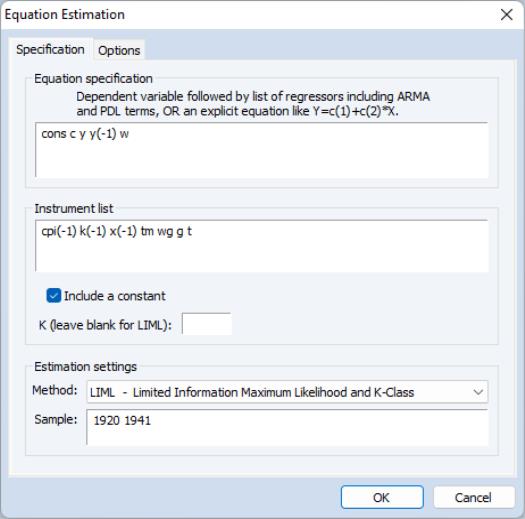
To estimate a LIML or K‑Class equation in EViews, create an equation by choosing or , and choose from the box.
Alternately, you may enter the keyword liml in the command window then hit ENTER.
In the edit box, specify your dependent variable and exogenous variables, and in the edit box, provide a list of instruments. Endogenous variables should be entered in both the box and the box.
For K-Class estimation, enter the value of

in the box labeled . If no value is entered in this box, LIML is performed.
If you wish to estimate a non-linear equation, then enter the expression for the non-linear equation in the box. Note that non-linear K-Class estimation is currently not permitted; only non-linear LIML may be performed.
If you do not wish to include a constant as one of the instruments, uncheck the checkbox.
Different standard error calculations may be chosen by changing the dropdown menu on the tab of the estimation dialog. Note that if your equation was non-linear, only IV based standard errors may be calculated. For linear estimation you may also choose K-Class based, Bekker, or Hansen, Hausman and Newey standard errors.
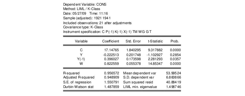
As an example of LIML estimation, we estimate part of Klein’s Model I, as published in Greene (2008, p. 385). We estimate the Consumption equation, where consumption (CONS) is regressed on a constant, private profits (Y), lagged private profits (Y(-1)), and wages (W) using data in the workfile “Klein.WF1”. The instruments are a constant, lagged corporate profits (P(-1)), lagged capital stock (K(-1)), lagged GNP (X(-1)), a time trend (TM), Government wages (WG), Government spending (G) and taxes (T). In his reproduction of the Klein model, Greene uses K‑Class standard errors. The results of this estimation are as follows:
EViews identifies the LIML estimation procedure, along with the choice of covariance matrix type and the list of instruments in the header. This information is followed by the usual coefficient, t-statistics, and asymptotic p-values.
The standard summary statistics reported at the bottom of the table are computed using the formulae outlined in
“Summary Statistics”. Along with the standard statistics, the LIML minimum eigenvalue is also reported, if the estimation type was LIML.


 , where y is the dependent variable, X are explanatory variables, and Z are instrumental variables.
  and
and  . Then the linear LIML objective function can be written as:
 be the smallest eigenvalue of
  . The LIML estimator of
  is the eigenvector corresponding to
  , with a normalization so that the first element of the eigenvector equals -1.
 are the regression residuals and
  .
. , given by:

 and
and  .
. , then the K-Class estimator is the TSLS estimator. If
  , then the K-Class estimator is OLS. LIML is a K-Class estimator with
  , the minimum eigenvalue described above.


 and
and  .
.
 in the box labeled K (leave blank for LIML). If no value is entered in this box, LIML is performed.