Principal components analysis.
Syntax
group_name.pcomp(options) [indices]
where the elements to display in loadings, scores, and biplot graph form (“out=loadings”, “out=scores” or “out=biplot”) are given by the optional indices, (e.g., “1 2 3” or “2 3”). If indices is not provided, the first two elements will be displayed.
Basic Options
out=arg (default=“table”) | Output type: eigenvector/eigenvalue table (“table”), eigenvalues graph (“graph”), loadings graph (“loadings”), scores graph (“scores”), biplot (“biplot”). |
eigval=vec_name | Specify name of vector to hold the saved the eigenvalues in workfile. |
eigvec=mat_name | Specify name of matrix to hold the save the eigenvectors in workfile. |
prompt | Force the dialog to appear from within a program. |
p | Print results. |
Number of Component Options
fsmethod=arg (default=“simple”) | Component retention method: “bn” (Bai and Ng (2002)), “ah” (Ahn and Horenstein (2013)), “simple” (simple eigenvalue methods), “user” (user-specified value). Note the following: (1) If using simple methods, the minimum eigenvalue and cumulative proportions may be specified using “minigen=” and “cproport=”. (2) If setting “fsmethod=user” to provide a user-specified value, you must specify the value with “r=”. |
r=arg (default=1) | User-specified number of components to retain (for use when “fsmethod=user”). |
mineigen=arg (default=0) | Minimum eigenvalue to retain component (when “fsmethod=simple”). |
cproport=arg (default=1.0) | Cumulative proportion of eigenvalue total to attain (when “fsmethod=simple”). |
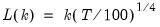
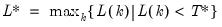
mfmethod=arg (default=“user”) | Maximum number of components used by selection methods: “schwert” (Schwert’s rule, default), “ah” (Ahn and Horenstein’s (2013) suggestion), “rootsize” ( 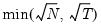 ), “size” (  ) ), “user” (user specified value), where  is the number of series and  is the number of observations. (1) For use with all components retention methods apart from user-specified (“fsmethod=user”). (2) If setting “mfmethod=user”, you may specify the maximum number of components using “rmax=”. (3) Schwert’s rule sets the maximum number of components using the rule: let for  and let and let  ; then the default maximum lag is given by ; then the default maximum lag is given by |
n=arg or rmax=arg (default=all) | User-specified maximum number of factors to retain (for use when “mfmethod=user”). |
fsic=arg (default=avg) | Component selection criterion (when “fsmethod=bn”): “icp1” (ICP1), “icp2” (ICP2), “icp3” (ICP3), “pcp1” (PCP1), “pcp2” (PCP1), “pcp3” (ICP3), “avg” (average of all criteria ICP1 through PCP3). Component selection criterion (when “fsmethod=ah”): “er” (eigenvalue ratio), “gr” (growth ratio), “avg” (average of eigenvalue ratio and growth ratio). Component selection (when “fsmethod=simple”): “min” (minimum of: minimum eigenvalue, cumulative eigenvalue proportion, and maximum number of factors), “max” (maximum of: minimum eigenvalue, cumulative eigenvalue proportion, and maximum number of factors), “avg” (average the optimal number of factors as specified by the min and max rule, then round to the nearest integer). |
demeantime | Demeans observations across time prior to component selection procedures, when “n=bn” or “n=ah”. |
sdizetime | Standardizes observations across time prior to component selection procedures, when “n=bn” or “n=ah”. |
demeancross | Demeans observations across cross-sections prior to component selection procedures, when “n=bn” or “n=ah”. |
sdizecross | Standardizes observations across cross-sections prior to component selection procedures, when “n=bn” or “n=ah”. |
Eigenvalues Plot Options
The default eigenvalue graph shows a scree plot of the ordered eigenvalues. You may use the “scree”, “cproport”, and “diff” option keywords to display any combination of the scree plot, cumulative eigenvalue proportions plot, or eigenvalue difference plot.
scree | Display a scree plot of the eigenvalues (if “output=graph). |
diff | Display a graph of the eigenvalue differences (if “output=graph). |
cproport | Display a graph of the cumulative proportions (if “output=graph). |
Loadings, Scores, Biplot Graph Options
scale=arg, (default= “normload”) | Diagonal matrix scaling of the loadings and the scores: normalize loadings (“normload”), normalize scores (“normscores”), symmetric weighting (“symmetric”), user-specified (arg=number). |
cpnorm | Compute the normalization for the scores so that cross-products match the target (by default, EViews chooses a normalization scale so that the moments of the scores match the target). |
nocenter | Do not center the elements in the graph. |
mult=arg (default=”first”) | Multiple graph options: first versus remainder (“first”), pairwise (“pair”), all pairs arrayed in lower triangle (“lt”) |
labels=arg (default=“outlier”) | Scores label options: identify outliers only (“outlier”), all points (“all”), none (“none”). |
labelprob=arg (default=0.1) | Outlier label probability (if “labels=outlier”). |
autoscale=arg (default=1.0) | Rescaling factor for auto-scaling. |
userscale=arg | User-specified scaling. |
Covariance Options
cov=arg (default=“corr”) | Covariance calculation method: ordinary (Pearson product moment) covariance (“cov”), ordinary correlation (“corr”), Spearman rank covariance (“rcov”), Spearman rank correlation (“rcorr”), uncentered ordinary correlation (“ucorr”). Note that Kendall’s tau measures are not valid methods. |
wgt=name (optional) | Name of series containing weights. |
wgtmethod=arg (default = “sstdev”) | Weighting method: frequency (“freq”), inverse of variances (“var”), inverse of standard deviation (“stdev”), scaled inverse of variances (“svar”), scaled inverse of standard deviations (“sstdev”). Only applicable for ordinary (Pearson) calculations where “weights=” is specified. Weights for rank correlation and Kendall’s tau calculations are always frequency weights. |
pairwise | Compute using pairwise deletion of observations with missing cases (pairwise samples). |
partial=arg | Compute partial covariances conditioning on the list of series specified in arg. |
df | Compute covariances with a degree-of-freedom correction accounting for the mean (for centered specifications) and any partial conditioning variables. The default behavior in these cases is to perform no adjustment ( e.g. – compute sample covariance dividing by  rather than  ). |
Examples
group g1 x1 x2 x3 x4
freeze(tab1) g1.pcomp(eigval=v1, eigvec=m1)
The first line creates a group named g1 containing the four series x1, x2, x3, x4. The second line produces a view of the basic results for the principal components. The output view is stored in a table named tab1, the eigenvalues in a vector named v1, and the eigenvectors in a matrix named m1.
g1.pcomp(out=graph)
g1.pcomp(out=graph, scree, cproport)
displays a screen plot of the eigenvalues, and a graph containing both a screen plot and a plot of the cumulative eigenvalue proportions.
g1.pcomp(out=loading)
displays a loadings plot, and
g1.pcomp(out=biplot, scale=symmetric, mult=lt) 1 2 3
displays a symmetric biplot for all three pairwise comparisons.
Cross-references
See
“Principal Components” for further discussion.
To save principal components scores in series in the workfile, see
Group::makepcomp.