Principal Components
Principal components analysis models the variance structure of a set of observed variables using linear combinations of the variables. These linear combinations, or components, may be used in subsequent analysis, and the combination coefficients, or loadings, may be used in interpreting the components. While we generally require as many components as variables to reproduce the original variance structure, we usually hope to account for most of the original variability using a relatively small number of components.
We may, for example, have a very large number of variables describing individual health status that we wish to reduce to a manageable set. By forming linear combinations of the observed variables we may achieve data reduction by creating a handful of measures that describe overall health (e.g., “strength,” “fitness,” “disabilities”). The coefficients in these linear combinations may be used to provide interpretation to the newly constructed health measures.
The principal components of a set of variables are obtained by computing the eigenvalue decomposition of the observed variance matrix. The first principal component is the unit-length linear combination of the original variables with maximum variance. Subsequent principal components maximize variance among unit-length linear combinations that are orthogonal to the previous components.
For additional details see Johnson and Wichtern (1992).
Performing Principal Components
EViews allows you to compute the principal components of the estimated correlation or covariance matrix of a group of series, and to display your results in a variety of ways. You may display the table of eigenvalues and eigenvectors, display line graphs of the ordered eigenvalues, and examine scatterplots of the loadings and component scores. Furthermore you may save the component scores and corresponding loadings to the workfile.
As an illustration, we again consider the stock price example from Johnson and Wichtern (1992) in which 100 observations on weekly rates of return for Allied Chemical, DuPont, Union Carbide, Exxon, and Texaco were examined over the period from January 1975 to December 1976 (“Stocks.WF1”).
To perform principal components on these data, we open the group G1 containing the series and select to open the dialog:
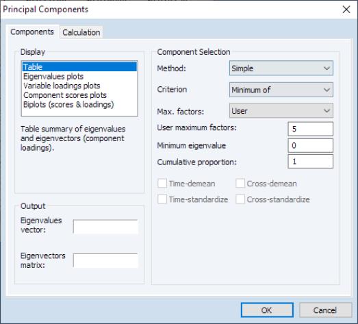
The principal components dialog has two tabs. Here, we have selected the first tab, labeled . The second tab, labeled controls the computation of the dispersion matrix from the series in the group. By default, EViews will perform principal components on the ordinary (Pearson)
correlation matrix, but you may use the settings on this tab to modify the preliminary calculation. We will examine this tab in greater detail in
“Covariance Calculation”.
Viewing the Components
The tab is used to specify options for displaying the components or saving the eigenvalues and eigenvectors of the variances.
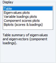
The box allows you to choose between showing the eigenvalues and eigenvectors in a tabular form, or displaying line graphs of the ordered eigenvalues, or scatterplots of the loadings, scores, or both (biplot). As you select different display methods, the remainder of the dialog will change to provide you with different settings.
Table
In the figure above, the display setting is chosen. There are two sets of fields that you may wish to modify.
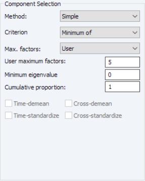
First, EViews provides you with a number of settings for controlling the number of components to be displayed.
The dropdown lets you choose between the , , and . In turn, each of these choices offers different options.
• If you select , you will choose a from the dropdown. You may choose from the following selections: , , .
For the first two selections, the number of factors is determined as the minimum or maximum of the (discussed below), the specified , and of eigenvalues. The will use the average of the other two results.
• If you select , EViews will employ the Bai and Ng (2002) method as discussed in
“Bai and Ng”.
The dropdown offers all of the information criteria described by Bai and Ng (, , , , , ) as well as the which averages the criteria prior to determining the optimal number of factors.
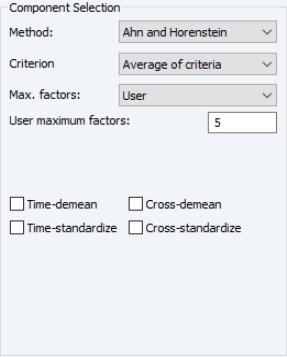
• If you select , EViews will compute the Ahn and Horenstein (2013) number of factor determination procedure (
“Ahn and Horenstein”). The dialog looks the same as for , but the dropdown now offers , , and .
• For , the number of factors is specified by the user in the edit box
In all of the automatic factor selection procedures above is the selection of maximum factors to be considered. While ultimately an arbitrary selection, EViews offers some suggestions typically seen in the literature. In particular, as in the case of ADF selection, l consider the dropdown which provides the following options:
• : let there be a lag choice function
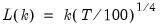
for
and let
; then returns the value
.
• : uses the suggestion made on page 1208 in Ahn and Horenstein (2013).
• : uses
.
• uses

.
• : users can specify an arbitrary value in the edit field.
Furthermore, as discussed in Bai and Ng (2002) and Ahn and Horenstein (2013), factor selection procedures can be improved dramatically if time and/or cross-section dimensions are demeaned and/or standardized. To allow for these possibilities, there are four checkboxes associated with each of these options and combinations:
• : demeans the time dimension.
• : standardizes the time dimension.
• : demeans the cross-section dimension.
• : standardizes the cross-section dimension.
The fields allow you to save the eigenvalues and eigenvectors to the workfile. Simply enter a valid name in the corresponding field if you wish EViews to save your results.
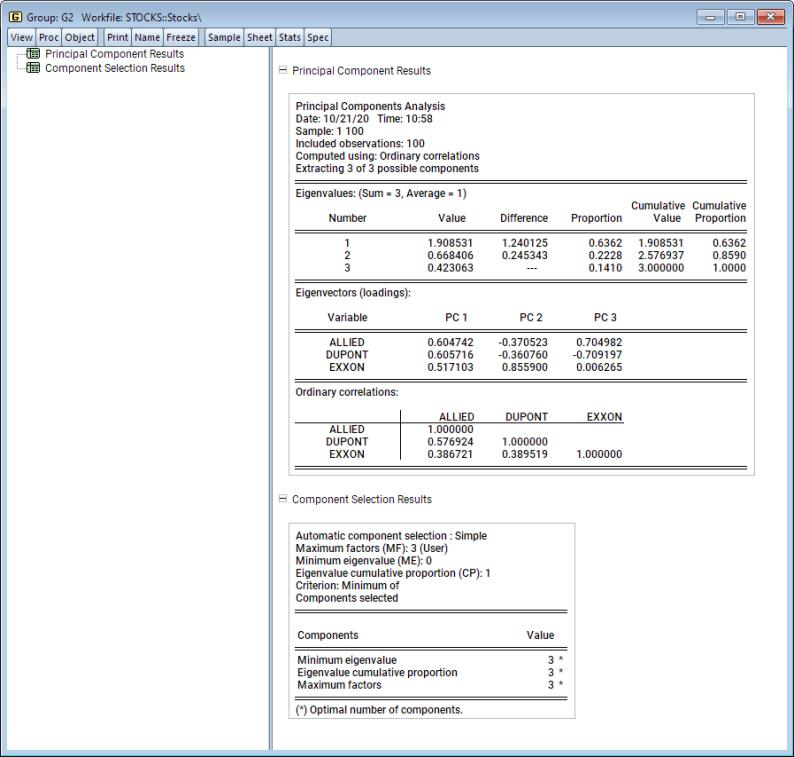
If we leave the default settings as is and click , EViews will display a spool containing the results of the principal components analysis and the results of the factor selection procedure:
The first node of the spool contains the table of principal components results:
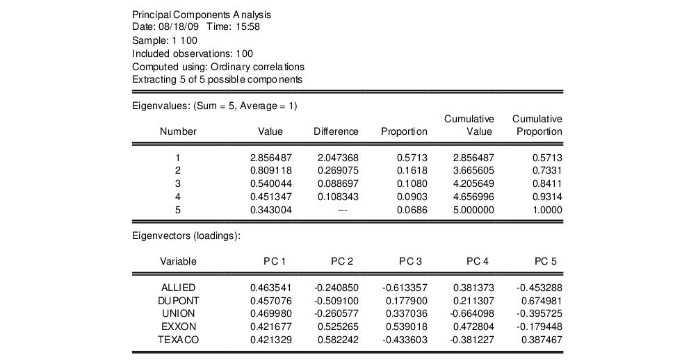
Here we show the top two sections of the table. The header describes the sample of observations, the method used to compute the dispersion matrix, and information about the number of components retained (in this case, all five).
The next section summarizes the eigenvalues, showing the values, the forward difference in the eigenvalues, the proportion of total variance explained, etc. Since we are performing principal components on a correlation matrix, the sum of the scaled variances for the five variables is equal to 5. The first principal component accounts for 57% of the total variance (2.856/5.00 = 0.5713), while the second accounts for 16% (0.809/5.00 = 0.1618) of the total. The first two components account for over 73% of the total variation.
The second section describes the linear combination coefficients. We see that the first principal component (labeled “PC1”) is a roughly-equal linear combination of all five of the stock returns; it might reasonably be interpreted as a general stock return index. The second principal component (labeled “PC2”) has negative loadings for the three chemical firms (Allied, du Pont and Union Carbide), and positive loadings for the oil firms (Exxon and Texaco). This loading appears to represent an industry specific component.
The third section of the output displays the calculated correlation matrix:
The second node contains results for the number of components selection procedure:
Here, we see that the number of components suggested for each of the simple criteria is 5. The overall criterion uses the minimum of the individual selections, and the number of components selected is also 5.
Eigenvalues Plots
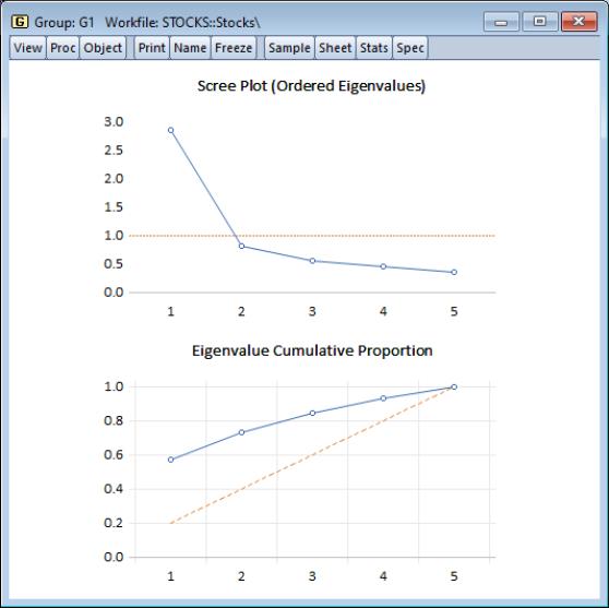
You may elect to display line graphs of the ordered eigenvalues by selecting in the portion of the main dialog. The dialog will change to offer you the choice of displaying plots of any of: the eigenvalues (scree plot), the eigenvalues difference, the cumulative proportion of variance explained. By default, EViews will only display the scree plot of ordered eigenvalues.
For the stock data, displaying the scree and cumulative proportion graphs yields the graph depicted here. The scree plot in the upper portion of the view shows the sharp decline between the first and second eigenvalues. Also depicted in the graph is a horizontal line marking the mean value of the eigenvalues (which is always 1 for eigenvalue analysis conducted on correlation matrices).
The lower portion of the graph shows the cumulative proportion of the total variance. As we saw in the table, the first two components account for about 73% of the total variation. The diagonal reference line offers an alternative method of evaluating the size of the eigenvalues. The slope of the reference line may be compared with the slope of the cumulative proportion; segments of the latter that are steeper than the reference line have eigenvalues that exceed the mean.
Other Graphs (Variable Loadings, Component Scores, Biplots)
The remaining three graphs selections produce graphs of the loadings (variables) and scores (observations): the variable loadings plots () produce component-wise plots of the eigenvectors (factor loading coefficients), allowing you to visualize the composition of the components in terms of the original variables; the scores plot () shows the actual values of the components for the observations in the sample; the biplot () combines the loadings and scores plots in one display.
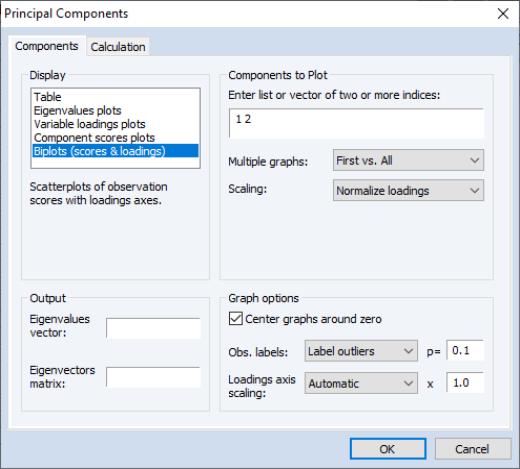
We continue our example by displaying the biplot graph since it includes the options for both the loadings and scores plots. If we select the entry, the right side of the dialog changes to provide additional plot options.
Components to Plot
The top right portion of the dialog, labeled is where you will provide the basic specification for the graphs that you want to display.
First, you must provide a list of components to plot. Here, the default setting “1 2” instructs EViews to place the first component on the x-axis and the second component on the y-axis. You may reverse the order of the axes by reversing the indices.
You may add indices for additional components. When more than two indices are provided, the setting provides choices for how you wish to process the indices. You may elect to plot the first listed component against the remaining components (), to use successive pairs of indices to form plots (), or to plot each component against the others ().
The options determine the weights to be applied to eigenvalues in the scores and the loadings (see
“Technical Discussion” for details). By default, the loadings are normalized so the observation scores have norms proportional to the eigenvalues (). You may instead choose to normalize the scores instead of the loadings () so that the observation score norms are proportional to unity, to apply symmetric weighting (), or to specify a user-supplied loading weight ().
In the latter three cases, you will be prompted to indicate whether you wish to adjust the results account for the sample size (). By default, EViews uses this setting and scales the loadings and scores so that the variances of the scores (instead of the norms) have the desired structure (see
“Observation Scaling”). Setting this option may improve the interpretability of the plot. For example, when normalizing scores, the weight adjustment scales the results so that the Euclidean distances between observations are the Mahalanobis distances and the cosines of the angles between variables are the covariances.
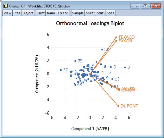
Using the default settings and clicking on , EViews produces the view:
The component scores are displayed as circles and the variable loadings are displayed as lines from the origin with variable labels. The biplot clearly shows us that the first component has positive loadings for all five variables (the general stock return index interpretation). The second component has positive variable loadings for the energy stocks, and negative loadings for the chemical stocks; when the energy stocks do well relative to the chemical stocks, the second specific component will be positive, and vice versa.
The scores labels show us that observation 3 is an outlier, with a high value for the general stock market index, and a relatively neutral value for the sector index. Observation 37 shows a poor return for the general market but is relatively sector neutral. In contrast, observation 20 is a period in which the overall market return was positive, with high returns to the energy sector relative to the chemical sector.
Graph Options
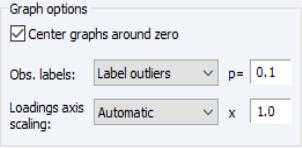
There are three additional options provided under . The first option is to . Unchecking this box will generally enlarge the graph within the frame at the expense of making it somewhat more difficult to quickly discern the signs of scores and loadings in a given dimension.
The dropdown allows you to choose the style of text labeling for observations. By default, EViews will , but you may instead choose to or to display . If you choose to label outliers, EViews will use a cutoff based on the specified probability value for the Mahalanobis distance of the observation from 0. The default is 0.1 so that labeled observations differ from the 0 with probability less than 0.1.
The last option, , is available only for biplot graphs. Note that the observations and variables in a biplot will generally have very different data scales. Instead of displaying biplots with dual scales, EViews applies a constant scaling factor to the loadings axes to make the graph easier-to-read. allows you to override the EViews default scale for the loadings in two distinct ways.
First, you may instruct EViews to apply a scale factor to the automatically chosen factor. This method is useful if you would like to stretch or shrink the EViews default axes. With the set to , simply enter your desired adjustment factor. The automatically determined loadings will be scaled by this factor.
Alternatively, if you wish to assign an absolute scaling factor, select for the axis scaling, and enter your scale factor. The original loadings will be scaled by this factor.
Saving Component Scores
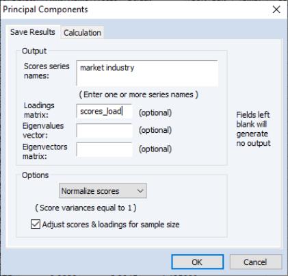
EViews provides easy-to-use tools for saving the principal components scores and scaled loadings matrices in the workfile. Simply select from the main group menu to display the dialog.
As with the main principal components view, the dialog has two tabs. The second tab controls the calculation of the dispersion matrix. The first describes the results that you wish to save.
The first option, , specifies the weights to be applied to eigenvalues in the scores and the loadings (see
“Technical Discussion” for details). By default, EViews will save the scores associated with normalized loadings (), but you may elect to save normalized scores (), equal weighted scores and loadings (), or user weighted loadings (), and the eigenvalues () and eigenvectors (). The default normalized loadings scores will have variances equal to the corresponding eigenvalues; the normalized scores will have unit variance.
For the latter three selections, you are also given the option of adjusting the scores and loadings for the sample size. If is selected, the scores are scaled so that their variance rather than the sums-of-squares (norms) match the desired value. In this example, the sample variances of the component scores will equal 1.
Next, you should enter names for the score series, one name per component score you wish to save. Here we enter two component names, “Market” and “Industry,” corresponding to the interpretation of our components given above. You may optionally save the loadings corresponding to the saved scores, eigenvalues, and eigenvectors to the workfile.
Covariance Calculation
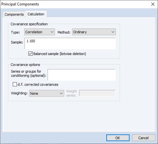
The EViews routines for principal components allow you to compute the dispersion matrix for the series in a group in a number of ways. Simply click on the tab to display the preliminary calculation settings.
The dropdown allows you to choose between computing a or a matrix.
The dropdown specifies computation of , , or , or measures. The selection dropdown is not applicable if you select or as your method.
The remaining settings should be familiar from the covariance analysis view (
“Covariance Analysis”). You may, for example, specify the sample of observations to be used and perform listwise exclusion of cases with missing values to balance the sample if necessary. Or you can perform partial and/or weighted analysis.
Note that component scores may not be computed for dispersion matrices estimated using Kendall’s tau-a and tau-b.
Technical Discussion
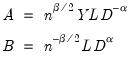
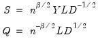
From the singular value decomposition, we may represent a

data matrix

of rank

as:
 | (12.27) |
where

and

are orthonormal matrices of the left and right singular vectors, and

is a diagonal matrix containing the singular values.
More generally, we may write:
 | (12.28) |
where

is an

, and

is a

matrix, both of rank

, and
 | (12.29) |
so that

is a factor which adjusts the relative weighting of the left (observations) and right (variables) singular vectors, and the terms involving

are scaling factors where

. The basic options in computing the scores

and the corresponding loadings

involve the choice of (loading) weight parameter

and (observation) scaling parameter

.
In the principal components context, let

be the cross-product moment (dispersion) matrix of

, and perform the eigenvalue decomposition:
 | (12.30) |
where

is the

matrix of eigenvectors and

is the diagonal matrix with eigenvalues on the diagonal. The eigenvectors, which are given by the columns of

, are identified up to the choice of sign. Note that since the eigenvectors are by construction orthogonal,
.
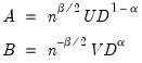
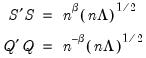
We may set

,

, and
, so that:
 | (12.31) |

may be interpreted as the
weighted principal components scores, and

as the
weighted principal components loadings. Then the scores and loadings have the following properties:
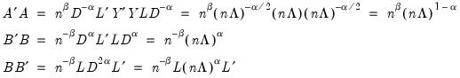 | (12.32) |
Through appropriate choice of the weight parameter

and the scaling parameter

, you may construct scores and loadings with various properties (see
“Loading Weights” and
“Observation Scaling”). EViews provides you with the opportunity to choose appropriate values for these parameters when displaying graphs of principal component scores and loadings and when saving scores and loadings to the workfile.
Note that when computing scores using
Equation (12.33), EViews will transform the

to match the data used in the original computation. For example, the data will be scaled for analysis of correlation matrices, and partialing will remove means and any conditioning variables. Similarly, if the preliminary analysis involves Spearman rank-order correlations, the data are transformed to ranks prior to partialing. Scores may not be computed for dispersion matrices estimated using Kendall’s tau.
Loading Weights
At one extreme, we define the
normalized loadings (also termed the
form, or
JK) decomposition where

. The scores formed from the normalized loadings decomposition will have variances equal to the corresponding eigenvalues. To see this, substituting into
Equation (12.31), and using
Equation (12.28) we have

, where:
 | (12.33) |
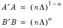
From
Equation (12.32), the scores

and loadings

have the norms:
 | (12.34) |
The rows of

are said to be in
principal coordinates, since the norm of

is the diagonal matrix with the eigenvalues on the diagonal. The columns of

are in
standard coordinates since

is orthonormal
(Aitchison and Greenwood, 2002, p. 378). The JK specification has a
row preserving metric (RPM) since the observations in

retain their original scale.
At the other extreme, we define the
normalized scores (also referred to as the
covariance or
GH) decomposition where

. Then we may write

where:
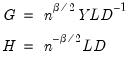 | (12.35) |
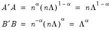
Evaluating the norms using
Equation (12.32), we have:
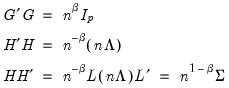 | (12.36) |
For this factorization,

is orthonormal (up to a scale factor) and the norm of

is proportional to the diagonal matrix with the

times the eigenvalues on the diagonal. Thus, the specification is said to favor display of the variables since the

loadings are in principal coordinates and the scores

are in standard coordinates (so that their variances are identical). The GH specification is sometimes referred to as the
column metric preserving (CMP) specification.
In interpreting results for the GH decomposition, bear in mind that the Euclidean distances between observations are proportional to Mahalanobis distances. Furthermore, the norms of the columns of

are proportional to the factor covariances, and the cosines of the angles between the vectors approximate the correlations between variables.
Obviously, there are an infinite number of alternative scalings lying between the extremes. One popular alternative is to weight the scores and the loadings equally by setting

: This specification is the
SQ or
symmetric biplot, where

:
 | (12.37) |
Evaluating the norms of the scores

and loadings

, we have:
 | (12.38) |
so that the norms of both the observations and the variables are proportional to the square roots of the eigenvalues.
Observation Scaling
In the decompositions above, we allow for observation scaling of the scores and loadings parameterized by

. There are two obvious choices for the scaling parameter

.
First, we could ignore sample size by setting

so that:
 | (12.39) |
With no observation adjustment, the norm of the scores equals

, the variance of the scores equals

, and the norm of the variables equals

times the eigenvalues raised to the

power. Note that the observed
variance of the scores is not equal to, but is instead proportional to

, and that the norm of the loadings is only proportional to

.
Alternately, we may set

, yielding:
 | (12.40) |
With this sample size adjustment, the variance of the scores equals

and the norm of the variables equals

.
Gabriel (1971), for example, recommends employing a
principal components decomposition for biplots that sets

. From
Equation (12.32) the relevant norms are given by:
 | (12.41) |
By performing observation scaling, the scores are normalized so that their variances (instead of their norms) are equal to 1. Furthermore the Euclidean distances between points are equal to the Mahalanobis distances (using

), the norms of the columns of

are equal to the eigenvalues, and the cosines of the angles between the vectors equal the correlations between variables. Without observation scaling, these results only hold up to a constant of proportionality.
By default, EViews performs observation scaling, setting

. To remove this adjustment, simply uncheck the checkbox. Note that when EViews performs this adjustment, it employs the denominator from the original dispersion calculation which will differ from

if any degrees-of-freedom adjustment has been applied.
Determining the Number of Components
The use of principal components factors has become an important feature of modern econometric analysis, with applications in areas such as data-rich forecasting, unit root testing, and VAR estimation.
A central task in using components (factors) is the choice of the number of factors to be employed in analysis. While there are a number of approaches to answering this question, we focus here on easy-to-compute methods that focus on eigenvalue heuristics, as well as data-driven approaches proposed by Bai and Ng (2002) and Ahn and Horenstein (2013).
Approaches to selecting numbers of components center around the idea of optimal dimensionality reduction. Recall that every

symmetric matrix

with rank

may be diagonalized orthogonally so that
 | (12.42) |
where
is the diagonalizing matrix spanned by the

-element eigenvectors

of

, and
is a diagonal matrix with elements

denoting the eigenvalues associated with the corresponding

.
Suppose, that we have data for

for variable

and periods

, respectively, and define the vectors and matrices
and
. When

is the covariance matrix of

, the diagonalization is an orthogonal decomposition of the correlation structure among the

variables. It turns out that this procedure also preserves that the correlation dynamics of the variables.
It can be shown that the linear combination of all

columns of

in the direction of

, termed the
i-th principal component or factor contributes to
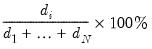 | (12.43) |
of total system variation. Accordingly, if we arrange the eigenvalues from largest to smallest, say
the corresponding principal components are arranged from most principal to least in the proportion of total system variation contributed by that direction.
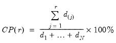
Dimensionality reduction may then be attained by discarding the

least important principal components until the desired degree of reduction is attained. The retained

principal components contribute to the cumulative proportion
 | (12.44) |
of the original variation in

.
Simple Rules
One approach to selecting the number of retained components is to use simple heuristics. The strategies discussed here, while in the spirit of optimal dimensionality reduction, rely entirely on arbitrarily selected criteria.
In particular, the following eigenvalue based rules are often employed to select

,
• Maximum components: specifies

directly and arbitrarily.
• Minimum eigenvalue: retained components must be associated with directions that have

for some arbitrary minimum

.
• Minimum eigenvalue cumulative proportion: retained components must have eigenvalues satisfying
 | (12.45) |
for a specified

. This rule retains the first

principal components that capture at least

% of the original variation.
Slightly more complex decision rules involve combinations of the three decision rules from above. Two very simple ones are:
• Minimum rule: selects the minimum number of components satisfying the three rules above.
• Maximum rule: selects the maximum number of components satisfying the three rules above.
Bai and Ng
Bai and Ng (2002) cast the number of components selection problem in terms of model selection. Consider the following factor model,
 | (12.46) |
where the cross-section data depends on a set of

common factors

and individual cross-section weights, or loadings,

. Note that the number of components is given by the number of elements of

.
Consider the optimization problem
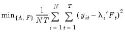 | (12.47) |
subject to the normalization
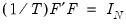
where

is the identity matrix,

is a

matrix of of
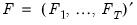
and

is a

matrix of variable specific of loadings
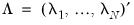
.
The factor matrix may be estimated as
 | (12.48) |
where

is the

matrix of the first

principal eigenvectors of

.
The corresponding loading matrix

is then estimated by regressing

on

, yielding
 | (12.49) |
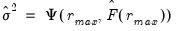
Since the objective is to identify the optimal number of factors, we would like to give consideration to the full set of possible outcomes. The maximum number of factors that can be estimated is
, so we consider
(though typically one imposes
for some known number

of maximum factors under consideration).
For a given

, we may define the objective function for obtaining loadings as the regression problem:
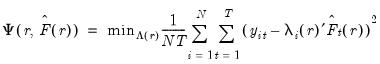 | (12.50) |
where

is the matrix of factors formed from the

largest eigenvalues, and then compare results for the different

using conventional model selection tools.
Bai and Ng (2002) propose six loss functions that yield consistent estimates of

. The first three employ the objective function in levels
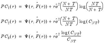 | (12.51) |
while the remainder use logarithms
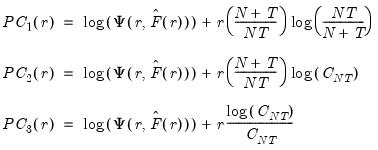 | (12.52) |
where
.
The selected optimal number of factors

is the

yielding the smallest loss function value.
Ahn and Horenstein
Ahn and Horenstein (AH, 2013) propose a method for obtaining the number of factors that exploits the fact that the

largest eigenvalues of a given matrix grow without bounds as the rank of the matrix increases, whereas the other eigenvalues remain bounded. The optimization strategy is then simply to find the maximum of the ratio of two adjacent eigenvalues. One of the advantages of this approach is that it is far less sensitive to the choice of

than is Bai and Ng (2002). Furthermore, the AH procedure is significantly easier to compute, requiring only the computation of eigenvalues.
As before, the model under consideration is given by:
 | (12.53) |
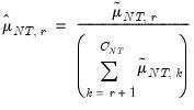
Let

denote the

-th largest eigenvalue of
. Further, define
 | (12.54) |
AH propose two estimators for the optimal number of factors. For optimal

where

, we have
• Eigenvalue ratio (ER)
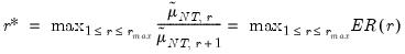 | (12.55) |
• Growth ratio (GR)
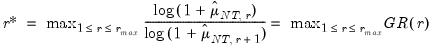 | (12.56) |
where
 | (12.57) |
Furthermore, AH propose a simple rule for selecting

:
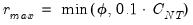 | (12.58) |
where
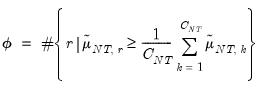 | (12.59) |
is the number of

for which

exceeds its average.
Lastly, we note that AH suggest that the data should be demeaned in both the time and cross-section dimensions. While this step is not necessary for consistency, it is useful in small samples. As a final caveat, AH warn against using their procedures in cases where some factors are

while others are

. When this is the case, factors should be differenced first, as in Bai and Ng (2004).