An Example Model
In this section, we demonstrate how we can use the EViews model object to implement a simple macroeconomic model of the U.S. economy. The specification of the model is taken from Pindyck and Rubinfeld (1998, p. 390). We have provided the data and other objects relating to the model in the sample workfile “Macromod.WF1”. You may find it useful to follow along with the steps in the example, and you can use the workfile to experiment further with the model object.
(A second, simpler example may be found in
“Plotting Probability Response Curves”).
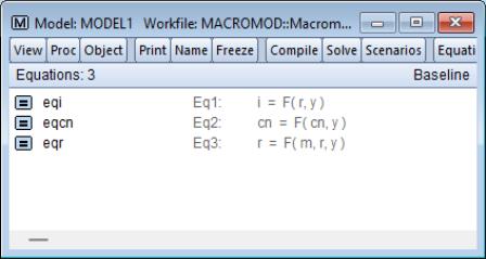
The macro model contains three stochastic equations and one identity. In EViews notation, these can be written:
cn = c(1) + c(2)*y + c(3)*cn(-1)
i = c(4) + c(5)*(y(-1)-y(-2)) + c(6)*y + c(7)*r(-4)
r = c(8) + c(9)*y + c(10)*(y-y(-1)) + c(11)*(m-m(-1)) + c(12)* (r(-1)+r(-2))
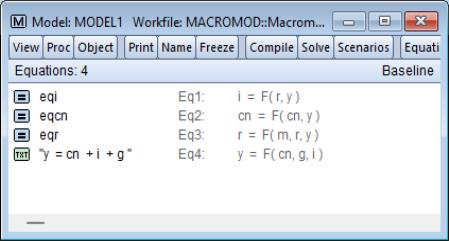
y = cn + i + g
where:
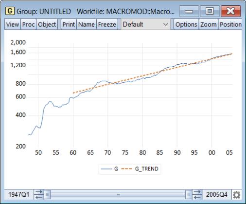
• CN is real personal consumption
• I is real private investment
• G is real government expenditure
• Y is real GDP less net exports
• R is the interest rate on three-month treasury bills
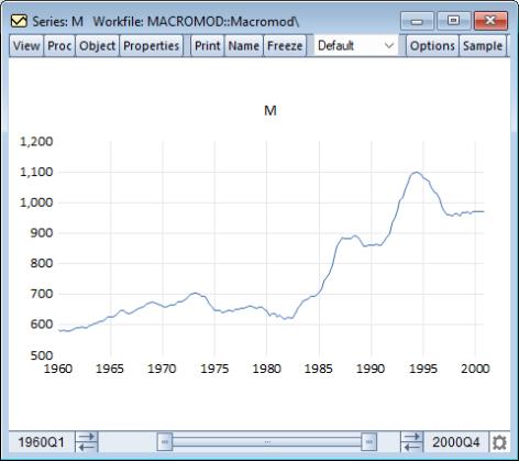
• M is the real money supply, narrowly defined (M1)
and the C(i) are the unknown coefficients.
The model follows the structure of a simple textbook ISLM macroeconomic model, with expenditure equations relating consumption and investment to GDP and interest rates, and a money market equation relating interest rates to GDP and the money supply. The fourth equation is the national accounts expenditure identity which ensures that the components of GDP add to total GDP. The model differs from a typical textbook model in its more dynamic structure, with many of the variables appearing in lagged or differenced form.
Estimating the Equations
To begin, we must first estimate the unknown coefficients in the stochastic equations. For simplicity, we estimate the coefficients by simple single equation OLS. Note that this approach is not strictly valid, since Y appears on the right-hand side of several of the equations as an independent variable but is endogenous to the system as a whole. Because of this, we would expect Y to be correlated with the residuals of the equations, which violates the assumptions of OLS estimation. To adjust for this, we would need to use some form of instrumental variables or system estimation (for details, see the discussion of single equation
“Two-stage Least Squares” and system
“Two-Stage Least Squares” and related sections beginning on
(here)).
To estimate the equations in EViews, we create three new equation objects in the workfile (using ), and then enter the appropriate specifications. Since all three equations are linear, we can specify them using list form. To minimize confusion, we will name the three equations according to their endogenous variables. The resulting names and specifications are:
Equation EQCN: | cn c y cn(-1) |
Equation EQI: | i c y(-1)-y(-2) y r(-4) |
Equation EQR: | r c y y-y(-1) m-m(-1) r(-1)+r(-2) |
The three equations estimate satisfactorily and provide a reasonably close fit to the data, although much of the fit probably comes from the lagged endogenous variables. The consumption and investment equations show signs of heteroskedasticity, possibly indicating that we should be modeling the relationships in log form. All three equations show signs of serial correlation. We will ignore these problems for the purpose of this example, although you may like to experiment with alternative specifications and compare their performance.
Creating the Model
Now that we have estimated the three equations, we can proceed to the model itself. To create the model, we simply select from the menus. To keep the model permanently in the workfile, we name the model by clicking on the button, enter the name MODEL1, and click on .
When first created, the model object defaults to equation view. Equation view allows us to browse through the specifications and properties of the equations contained in the model. Since we have not yet added any equations to the model, this window will appear empty.
Linking the Equations
To add our estimated stochastic equations to the model, we can simply copy-and-paste or drag-and-drop them from the workfile window. To copy-and-paste, first select the objects in the workfile window, and then use or the right mouse button menu to copy the objects to the clipboard. Click anywhere in the model object window, and use or the right mouse button menu to paste the objects into the model object window. To drag-and-drop, simply select the equation objects, then drag into the model window. Click on when prompted to link the equation to the object.
Alternatively, we could have combined the two steps by first highlighting the three equations, right-mouse clicking, and selecting . EViews will create a new unnamed model containing the three equations. Press on the button to name the model object.
The three estimated equations should now appear in the equation window. Each equation appears on a line with an icon showing the type of object, its name, its equation number, and a symbolic representation of the equation in terms of the variables that it contains. Double clicking on any equation will bring up a dialog of properties of that equation. For the moment, we do not need to alter any of these properties.
We have added our three equations as linked equations. This means if we go back and reestimate one or more of the equations, we can automatically update the equations in the model to the new estimates by using the procedure .
Adding the Identity
To complete the model, we must add our final equation, the national accounts expenditure identity. There is no estimation involved in this equation, so instead of including the equation via a link to an external object, we merely add the equation as inline text.
To add the identity, we click with the right mouse button anywhere in the equation window, and select . A dialog box will appear titled which contains a text box with the heading . Simply type the identity, “Y = CN + I + G”, into the text box, then click on to add it to the model.
The equation should now appear in the model window. The appearance differs slightly from the other equations, which is an indicator that the new equation is an inline text equation rather than a link.
Our model specification is now complete. At this point, we can proceed straight to solving the model.
Performing a Static Solution
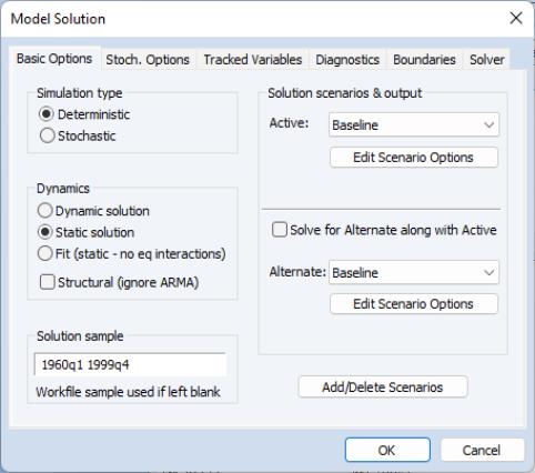
To solve the model, simply click on the button in the model window button bar.
There are many options available from the dialog, but for the moment we will consider only the basic settings. As our first exercise in assessing our model, we would like to examine the ability of our model to provide one-period ahead forecasts of our endogenous variables. To do this, we can look at the predictions of our model against our historical data, using actual values for both the exogenous and the lagged endogenous variables of the model. In EViews, we refer to this as a static simulation. We may easily perform this type of simulation by choosing in the box of the dialog.
We must also adjust the sample over which to solve the model, so as to avoid initializing our solution with missing values from our data. Most of our series are defined over the range of 1947Q1 to 1999Q4, but our money supply series is available only from 1959Q1. Because of this, we set the sample to 1960Q1 to 1999Q4, allowing a few extra periods prior to the sample for any lagged variables.
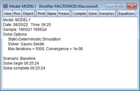
We are now ready to solve the model. Simply click on to start the calculations. The model window will switch to the view.
The output should be fairly self-explanatory. In this case, the solution took less than a second and there were no errors while performing the calculations.
Examining the Solution Results
Now that we have solved the model, we would like to look at the results. When we solved the model, the results for the endogenous variables were placed into series in the workfile with names determined by the name aliasing rules of the model. Since these series are ordinary EViews objects, we could use the workfile window to open the series and examine them directly. However, the model object provides a much more convenient way to work with the series through a view called the .
The easiest way to switch to the variable view is to select or to click on the button labeled on the model window button bar.
In the variable view, each line in the window is used to represent a variable. The line contains an icon indicating the variable type (endogenous, exogenous or add factor), the name of the variable, the equation with which the variable is associated (if any), and the description field from the label of the underlying series (if available). The name of the variable may be colored according to its status, indicating whether it is being traced (blue) or whether it has been overridden (red). In our model, we can see that CN, I, R and Y are endogenous variables in the model, while G and M are exogenous.
Much of the convenience of the variable view comes from the fact that it allows you to work directly with the names of the variables in the model, rather than the names of series in the workfile. This is useful because when working with a model, there are different series associated with each variable. For endogenous variables, there will be the actual historical values and one or more series of solution values. For exogenous variables, there may be several alternative scenarios for the variable. The variable view and its associated procedures help you move between these different sets of series without having to worry about the many different names involved.
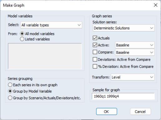
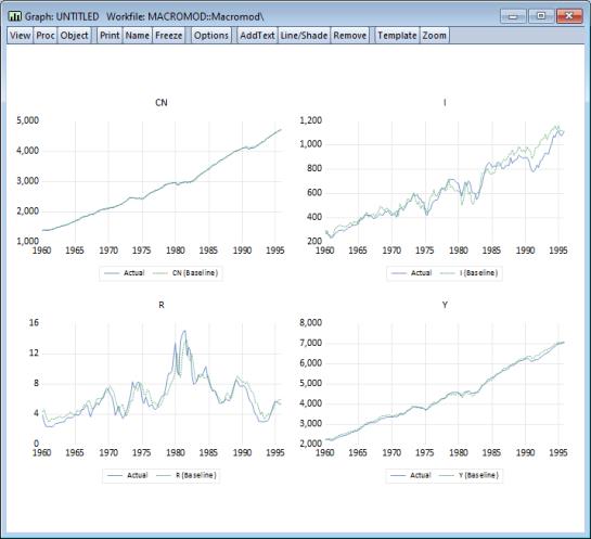
For example, to look at graphs containing the actual and fitted values for the endogenous variables in our model, we select the four variables (by holding down the control key and clicking on the variable names), then use to enter the dialog.
(The names of the four series will be pre-filled in the section. Alternately, we could have simply selected then set the dropdown to s.)
Again, the dialog has many options, but for our current purposes, we can leave most settings at their default values. Simply make sure that the and checkboxes are checked, set the sample for the graph to “1960 1999”, then click on .
The graphs show that as a one-step ahead predictor, the model performs quite well, although the ability of the model to predict investment deteriorates during the second half of the sample.
Performing a Dynamic Solution
An alternative way of evaluating the model is to examine how the model performs when used to forecast many periods into the future. To do this, we must use our forecasts from previous periods, not actual historical data, when assigning values to the lagged endogenous terms in our model. In EViews, we refer to such a forecast as a dynamic forecast.
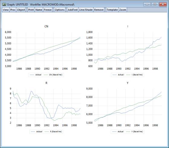
To perform a dynamic forecast, we will the model with a slightly different set of options. Return to the model window and again click on the button. In the model solution dialog, choose in the section of the dialog, and set the solution sample to “1985 1999”.
Click on to solve the model. To examine the results, we will use exactly as above to display the actuals and the baseline solutions for the endogenous variables. Make sure the sample is set to 1985Q1 to 1999Q4 then click on . The results illustrate how our model would have performed if we had used it back in 1985 to make a forecast for the economy over the next fifteen years, assuming that we had used the correct paths for the exogenous variables (in reality, we would not have known these values at the time the forecasts were generated). Not surprisingly, the results show substantial deviations from the actual outcomes, although they do seem to follow the general trends in the data.
Forecasting
Once we are satisfied with the performance of our model against historical data, we can use the model to forecast future values of our endogenous variables. The first step in producing such a forecast is to decide on values for our exogenous variables during the forecast period. These may be based on our best guess as to what will actually happen, or they may be simply one particular possibility that we are interested in considering. Often we will be interested in constructing several different paths and then comparing the results.
Filling in Exogenous Data
In our model, we must provide future values for our two exogenous variables: government expenditure (G), and the real money supply (M). For our example, we will try to construct a set of paths that broadly follow the trends of the historical data.
A quick look at our historical series for G suggests that the growth rate of G has been fairly constant since 1960, so that the log of G roughly follows a linear trend. Where G deviates from the trend, the deviations seem to follow a cyclical pattern.
As a simple model of this behavior, we can regress the log of G against a constant and a time trend, using an AR(4) error structure to model the cyclical deviations. This gives an equation object, which we save in the workfile as EQG, with the representation:
log(g) = 6.252335363 + 0.004716422189*@trend + [ar(1)=1.169491542,ar(2)=0.1986105964,ar(3)=0.239913126,ar(4)=-0.2453607091]
To produce a set of future values for G, we can use this equation to perform a dynamic forecast for G from 2000Q1 to 2005Q4, saving the results back into G itself; see
“Forecasting from an Equation” for details. Later we will show you how to instruct the model to use the data in a different series, say G_1, in place of the data in G (
“Using Scenarios for Alternate Assumptions”), so that you may preserve the original state of the series G.
The historical path of the real M1 money supply, M, is quite different from G, showing spurts of growth followed by periods of stability. For now, we will assume that the real money supply simply remains at its last observed historical value over the entire forecast period.
We can use an EViews series statement to fill in this path for the post 1999 period. The following lines will fill the series M from 2000Q1 to the last observation in the sample with the last observed historical value for M:
smpl 2000q1 @last
series m = m(-1)
smpl @all
We now have a set of possible values for our exogenous variables over the forecast period.
Producing Endogenous Forecasts
To produce forecasts for our endogenous variables, we return to the model window, click on , choose , set the forecast sample for 2000Q1 to 2005Q4, and then click on . The Solution Messages screen should appear, indicating that the model was successfully solved.
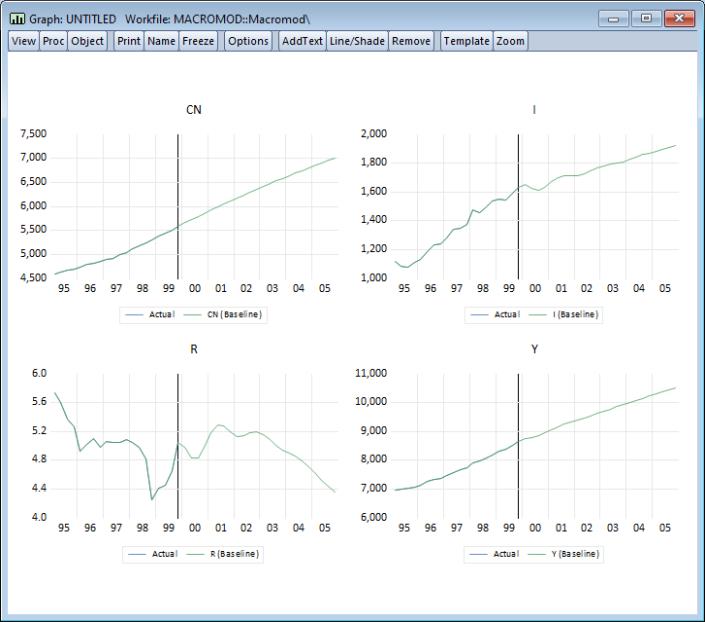
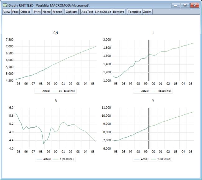
To examine the results in a graph, we again use from the variables view, select in the section, then set the sample to 1995Q1 to 2005Q4 (so that we include five years of historical data). We will only display the baseline results so uncheck the box, then click on to produce the graphs.
Click on the middle of the graph and select . After adding a line in 1999Q4 to separate historical and actual results, we get a graph showing the results:
We observe strange behavior in the results. At the beginning of the forecast period, we see a heavy dip in investment, GDP, and interest rates. This is followed by a series of oscillations in these series with a period of about a year, which die out slowly during the forecast period. This is not a particularly convincing forecast.
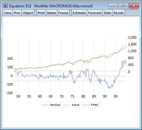
There is little in the paths of our exogenous variables or the history of our endogenous variables that would lead to this sharp dip, suggesting that the problem may lie with the residuals of our equations. Our investment equation is the most likely candidate, as it has a large, persistent positive residual near the end of the historical data (see figure below). This residual will be set to zero over the forecast period when solving the model, which might be the cause of the sudden drop in investment at the beginning of the forecast.
Using Add Factors to Model Equation Residuals
One way of dealing with this problem would be to change the specification of the investment equation. The simplest modification would be to add an autoregressive component to the equation, which would help reduce the persistence of the error. A better alternative would be to try to modify the variables in the equation so that the equation can provide some explanation for the sharp rise in investment during the 1990s.
An alternative approach to the problem is to leave the equation as it is, but to include an add factor in the equation so that we can model the path of the residual by hand. To include the add factor, we switch to the equation view of the model, double click on the investment equation, EQI, select the tab. Under Factor type, choose Equation intercept (residual shift). A prompt will appear asking if we would like to create the add factor series (if the series I_A does not already exist in the workfile). Click on to create the series. When you return to the variable view, you should see that a new variable, I_A, has been added to the list of variables in the model.
Using the add factor, we can specify any path we choose for the residual of the investment equation during the forecast period. By examining the view from the equation object, we see that near the end of the historical data, the residual appears to be hovering around a value of about 160. We will assume that this value holds throughout the forecast period. We can set the add factor using a few simple EViews commands:
smpl 2000q1 @last
i_a = 160
smpl @all
With the add factor in place, we can follow exactly the same procedure that we followed above to produce a new set of solutions for the model and a new graph for the results.
Including the add factor in the model has made the results far more appealing. The sudden dip in the first period of the forecast that we saw above has been removed. The oscillations are still apparent, but are much less pronounced.
Performing a Stochastic Simulation
So far, we have been working under the assumption that our stochastic equations hold exactly over the forecast period. In reality, we would expect to see the same sort of errors occurring in the future as we have seen in history. We have also been ignoring the fact that some of the coefficients in our equations are estimated, rather than fixed at known values. We may like to reflect this uncertainty about our coefficients in some way in the results from our model.
We can incorporate these features into our EViews model using stochastic simulation.
Up until now, we have thought of our model as forecasting a single point for each of our endogenous variables at each observation. As soon as we add uncertainty to the model, we should think instead of our model as predicting a whole distribution of outcomes for each variable at each observation. Our goal is to summarize these distributions using appropriate statistics.
If the model is linear (as in our example) and the errors are normal, then the endogenous variables will follow a normal distribution, and the mean and standard deviation of each distribution should be sufficient to describe the distribution completely. In this case, the mean will actually be equal to the deterministic solution to the model. If the model is not linear, then the distributions of the endogenous variables need not be normal. In this case, the quantiles of the distribution may be more informative than the first two moments, since the distributions may have tails which are very different from the normal case. In a non-linear model, the mean of the distribution need not match up to the deterministic solution of the model.
EViews makes it easy to calculate statistics to describe the distributions of your endogenous variables in an uncertain environment. To simulate the distributions, the model object uses a Monte Carlo approach, where the model is solved many times with pseudo-random numbers substituted for the unknown errors at each repetition. This method provides only approximate results. However, as the number of repetitions is increased, we would expect the results to approach their true values.
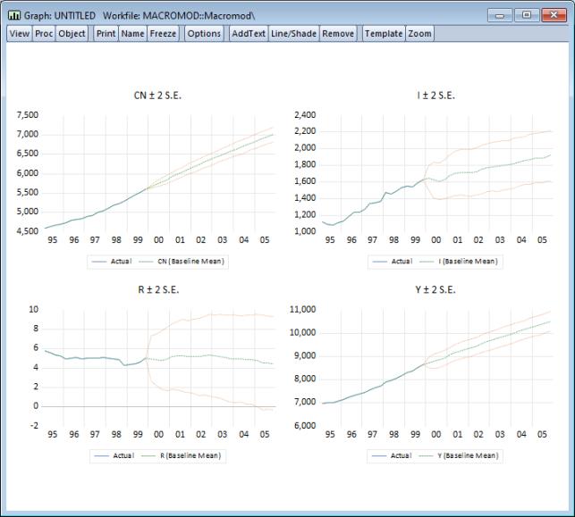
To return to our simple macroeconomic model, we can use a stochastic simulation to provide some measure of the uncertainty in our results by adding error bounds to our predictions. From the model window, click on the button. When the model solution dialog appears, choose for the simulation type and choose solution for the sample “2000 2005”. In the box on the right-hand side of the dialog, make sure that the checkbox in the section is checked. Click on to begin the simulation.
Status messages will appear to indicate progress of the simulation. When the simulation is complete select to display the results. As before, we will set the to and the sample to “1995 2005”. In addition, you should choose in the box, check the and scenario boxes, and set the latter to . Click on to produce the graph.
The error bounds in the resulting output graph show that we should be reluctant to place too much weight on the point forecasts of our model, since the bounds are quite wide on several of the variables. Much of the uncertainty is probably due to the large residual in the investment equation, which is creating a lot of variation in investment and interest rates in the stochastic simulation.
Using Scenarios for Alternate Assumptions
Another exercise we might like to consider when working with our model is to examine how the model behaves under alternative assumptions with respect to the exogenous variables. One approach to this would be to directly edit the exogenous series so that they contain the new values, and then resolve the model, overwriting any existing results. The problem with this approach is that it makes it awkward to manage the data and to compare the different sets of outcomes.
EViews provides a better way of carrying out exercises such as this through the use of model scenarios. Using a model scenario, you can override a subset of the exogenous variables in a model to give them new values, while using the values stored in the actual series for the remainder of the variables. When you solve for a scenario, the values of the endogenous variables are assigned into workfile series with an extension specific to that scenario, making it easy to keep multiple solutions for the model within a single workfile.
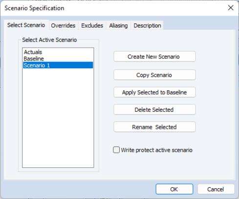
To create a scenario, we begin by selecting from the model object menus. The dialog will appear with a list of the scenarios currently defined in the model. You can use this dialog to select which scenario is currently active, or to create, rename, copy, and delete scenarios.
There are two special scenarios that are always present in the model: and . These two scenarios are special in that they cannot contain any overridden variables. The two scenarios differ in that the “Actuals” scenario writes its solution values directly into the workfile series with the same names as the endogenous variables, while the “Baseline” scenario writes its solution values back into workfile series with the names appended by the extension “_0”.
To add a new scenario to the model, simply click on the button labeled Create New Scenario. A new scenario will be created with the default name “Scenario 1”. Once we have created the scenario, we can modify the scenario from the baseline settings by overriding one of our exogenous variables. To add an override for the series M, first make certain that “Scenario 1” is active (highlighted in the dialog) then click on the Overrides tab and enter “M” in the dialog. Click on to accept your changes.
Alternately, after exiting the dialog, you may to return to the variable window of the model, click on the variable M, use the right mouse button to call up the dialog for the variable, and then in the box, click on the checkbox for. A message will appear asking if you would like to create the new series. Click on Yes to create the series, then to return to the variable window.
In the variable window, the variable name “M” should now appear in red, indicating that it has been overridden in the active scenario. This means that the variable M will now be bound to the series M_1 instead of the series M when solving the model using “Scenario 1”.
(You may use the tab to change the extension from “_1”. Note also that depending on how you created the override, you may still need to create the series M_1 in your workfile by copying the values of M.)
For example, in our previous forecast for M, we assumed that the real money supply would be kept at a constant level during the forecast period. For our alternative scenario, we are going to assume that the real money supply is contracted sharply at the beginning of the forecast period, and held at this lower value throughout the forecast. We can set the new values using a few simple commands:
smpl 2000q1 2005q4
series m_1 = 900
smpl @all
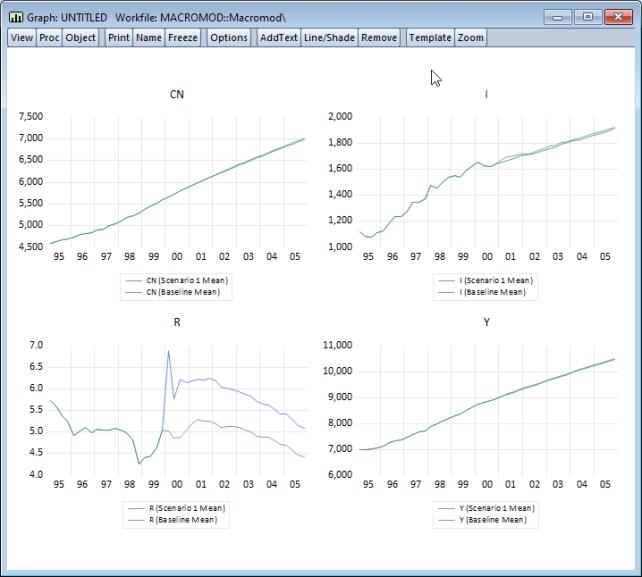
As before, we can solve the model by clicking on the button. Restore the to deterministic, make sure that “Scenario 1” is the active scenario, and “Baseline” is the alternate scenario, and that is checked. Set the solution sample to “2000 2005”. Click on to solve.
Once the solution is complete, we can use to display the results following the same procedure as above. First, set the selection to display the . Next, set the list box to the setting , then check both the and solution check boxes, making sure that the active scenario is set to “Scenario 1”, and the comparison scenario is set to “Baseline”. Set the sample to 1995Q1 to 2005Q4, then click on . The following graph should be displayed:
The simulation results suggest that the cut in the money supply causes a substantial increase in interest rates, which creates a small reduction in investment and a relatively minor drop in income and consumption. Overall, the predicted effects of changes in the money supply on the real economy are relatively minor in this model.
This concludes the discussion of our example model. The remainder of this chapter provides detailed information about working with particular features of the EViews model object.