Estimating a Panel Equation
The first step in estimating a panel equation is to call up an equation dialog by clicking on or from the main menu, or typing the keyword equation in the command window. You should make certain that your workfile is structured as a panel workfile. EViews will detect the presence of your panel structure and in place of the standard equation dialog will open the panel dialog.
You should use the dropdown menu to choose between , , and techniques. If you select the either of the latter two methods, the dialog will be updated to provide you with an additional page for specifying instruments (see
“Instrumental Variables Estimation”).
The remaining estimation supported estimation techniques do not account for the panel structure of your workfile, save for lags not crossing the boundaries between cross-section units.
Least Squares Estimation
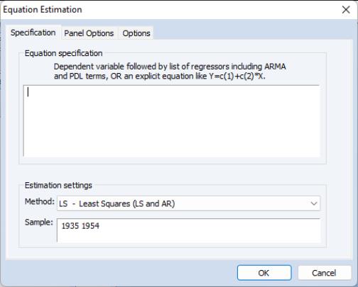
The basic least squares estimation dialog is a multi-page dialog with pages for the basic specification, panel estimation options, and general estimation options.
Least Squares Specification
You should provide an equation specification in the upper edit box, and an estimation sample in the edit box.
The equation may be specified by list or by expression as described in
“Specifying an Equation in EViews”.
In general, most of the specifications allowed in non-panel equation settings may also be specified here. You may, for example, include AR terms in both linear and nonlinear specifications, and may include PDL terms in equations specified by list. You may not, however, include MA terms in a panel setting.
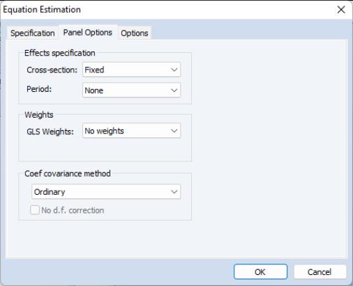
Least Squares Panel Options
Next, click on the tab to specify additional panel specific estimation settings.
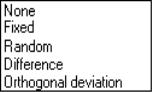
First, you should account for individual and period effects using the
Effects specification dropdown menus. By default, EViews assumes that there are no effects so that both dropdown menus are set to . You may change the default settings to allow for either or effects in either the cross-section or period dimension, or both. See the pool discussion of
“Fixed and Random Effects” for details.
You should be aware that when you select a fixed or random effects specification, EViews will automatically add a constant to the common coefficients portion of the specification if necessary, to ensure that the effects sum to zero.
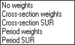
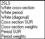
Next, you should specify settings for . You may choose to estimate with no weighting, or with , , , . The setting allows for contemporaneous correlation between cross-sections (clustering by period), while the allows for general correlation of residuals across periods for a specific cross-section (clustering by individual). and allow for heteroskedasticity in the relevant dimension.
For example, if you select , EViews will estimate a feasible GLS specification assuming the presence of cross-section heteroskedasticity. If you select , EViews estimates a feasible GLS specification correcting for heteroskedasticity and contemporaneous correlation. Similarly, allows for period heteroskedasticity, while corrects for heteroskedasticity and general correlation of observations within a cross-section. Note that the SUR specifications are both examples of what is sometimes referred to as the Parks estimator. See the pool discussion of
“Generalized Least Squares” for additional details.
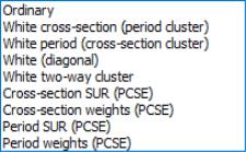
Lastly, you should specify a method for computing coefficient covariances. You may use the dropdown menu labeled to select from the various robust methods available for computing the coefficient standard errors. The covariance calculations may be chosen to be robust under various assumptions, for example, general correlation of observations within a cross-section, or perhaps cross-section heteroskedasticity. Select for one-way period clustering, for one-way cross-section clustering, for unstructured heteroskedasticity robust covariances, or for clustering by both cross-section and period. Click on the checkbox to perform the calculations without the leading degree of freedom correction term.
Each of the coefficient covariance methods is described in greater detail in
“Robust Coefficient Covariances”.
You should note that some combinations of specifications and estimation settings are not currently supported. You may not, for example, estimate random effects models with cross-section specific coefficients, AR terms, or weighting. Furthermore, while two-way random effects specifications are supported for balanced data, they may not be estimated in unbalanced designs.
LS Options
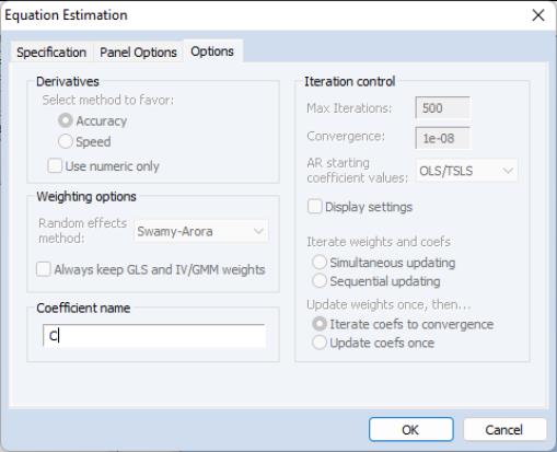
Lastly, clicking on the tab in the dialog brings up a page displaying computational options for panel estimation. Settings that are not currently applicable will be grayed out.
These options control settings for derivative taking, random effects component variance calculation, coefficient usage, iteration control, and the saving of estimation weights with the equation object.
These options are identical to those found in pool equation estimation, and are described in considerable detail in
“Options”.
Instrumental Variables Estimation
To estimate a pool specification using instrumental variables techniques, you should select in the dropdown menu at the bottom of the main () dialog page. EViews will respond by creating a four page dialog in which the third page is used to specify your instruments.
While the three original pages are unaffected by this choice of estimation method, note the presence of the new third dialog page labeled , which you will use to specify your instruments. Click on the tab to display the new page.
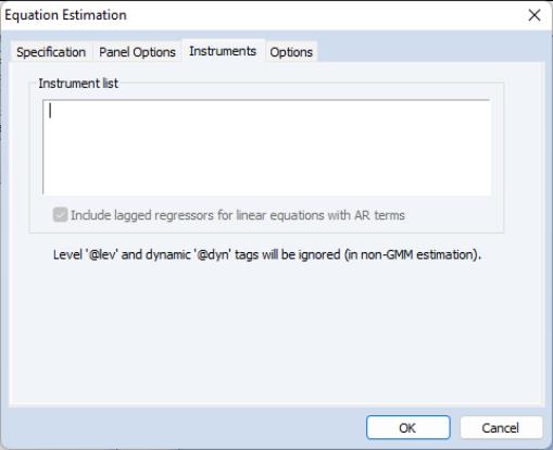
IV Instrument Specification
There are only two parts to the instrumental variables page. First, in the edit box labeled , you will list the names of the series or groups of series you wish to use as instruments.
Next, if your specification contains AR terms, you should use the checkbox to indicate whether EViews should automatically create instruments to be used in estimation from lags of the dependent and regressor variables in the original specification. When estimating an equation specified by list that contains AR terms, EViews transforms the linear model and estimates the nonlinear differenced specification. By default, EViews will add lagged values of the dependent and independent regressors to the corresponding lists of instrumental variables to account for the modified specification, but if you wish, you may uncheck this option.
See the pool chapter discussion of
“Instrumental Variables” for additional detail.
GMM Estimation
To estimate a panel specification using GMM techniques, you should select in the dropdown menu at the bottom of the main () dialog page. Again, you should make certain that your workfile has a panel structure. EViews will respond by displaying a four page dialog that differs significantly from the previous dialogs.
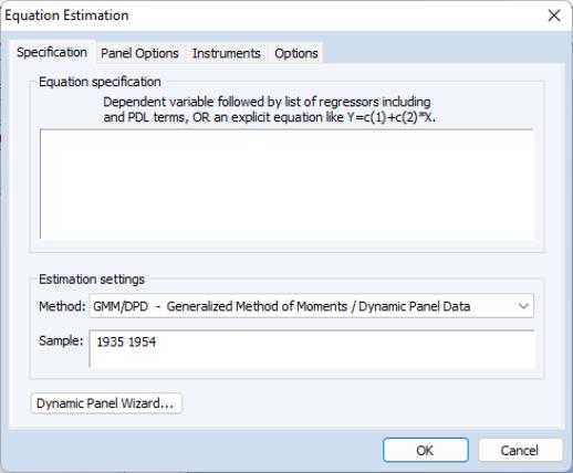
GMM Specification
The specification page is similar to the earlier dialogs. As in the earlier dialogs, you will enter your equation specification in the upper edit box and your sample in the lower edit box.
Note, however, the presence of the button on the bottom of the dialog. Pressing this button opens a wizard that will aid you in filling out the dialog so that you may employ dynamic panel data techniques such as the Arellano-Bond 1-step estimator for models with lagged endogenous variables and cross-section fixed effects. We will return to this wizard shortly (
“GMM Example”).
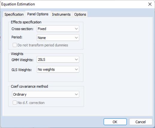
GMM Panel Options
Next, click on the dialog to specify additional settings for your estimation procedure.
As before, the dialog allows you to indicate the presence of cross-section or period fixed and random effects, to specify GLS weighting, and coefficient covariance calculation methods.
There are, however, notable changes in the available settings.
First, when estimating with GMM, there are two additional choices for handling cross-section fixed effects. These choices allow you to indicate a transformation method for eliminating the effect from the specification.
You may select to indicate that the estimation procedure should use first differenced data (as in Arellano and Bond, 1991), and you may use (Arellano and Bover, 1995) to perform an alternative method of removing the individual effects.
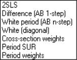
Second, the dialog presents you with a new dropdown menu so that you may specify weighting matrices that may provide for additional efficiency of GMM estimation under appropriate assumptions. Here, the available options depend on other settings in the dialog.
In most cases, you may select a method that computes weights under one of the assumptions associated with the robust covariance calculation methods (see
“Least Squares Panel Options”). If you select , for example, EViews uses GMM weights that are formed assuming that there is contemporaneous correlation between cross-sections.
If, however, you account for cross-section fixed effects by performing first difference estimation, EViews provides you with a modified set of GMM weights choices. In particular, the weights are those associated with the difference transformation. Selecting these weights allows you to estimate the GMM specification typically referred to as Arellano-Bond 1-step estimation. Similarly, you may choose the weights if you wish to compute Arellano-Bond 2-step or multi-step estimation. Note that the White period weights have been relabeled to indicate that they are typically associated with a specific estimation technique.
Note also that if you estimate your model using difference or orthogonal deviation methods, some GMM weighting methods will no longer be available.
GMM Instruments
Instrument specification in GMM estimation follows the discussion above with a few additional complications.
First, you may enter your instrumental variables as usual by providing the names of series or groups in the edit field. In addition, you may tag instruments as period-specific predetermined instruments, using the @dyn keyword, to indicate that the number of implied instruments expands dynamically over time as additional predetermined variables become available.
To specify a set of dynamic instruments associated with the series X, simply enter “@DYN(X)” as an instrument in the list. EViews will, by default, use the series X(-2), X(-3), ..., X(-T), as instruments for each period (where available). Note that the default set of instruments grows very quickly as the number of periods increases. With 20 periods, for example, there are 171 implicit instruments associated with a single dynamic instrument. To limit the number of implied instruments, you may use only a subset of the instruments by specifying additional arguments to @dyn describing a range of lags to be used.
For example, you may limit the maximum number of lags to be used by specifying both a minimum and maximum number of lags as additional arguments. The instrument specification:
@dyn(x, -2, -5)
instructs EViews to include lags of X from 2 to 5 as instruments for each period.
If a single argument is provided, EViews will use it as the minimum number of lags to be considered, and will include all higher ordered lags. For example:
@dyn(x, -5)
includes available lags of X from 5 to the number of periods in the sample.
Second, in specifications estimated using transformations to remove the cross-section fixed effects (first differences or orthogonal deviations), use may use the @lev keyword to instruct EViews to use the instrument in untransformed, or level form. Tagging an instrument with “@LEV” indicates that the instrument is for the transformed equation If @lev is not provided, EViews will transform the instrument to match the equation transformation.
If, for example, you estimate an equation that uses orthogonal deviations to remove a cross-section fixed effect, EViews will, by default, compute orthogonal deviations of the instruments provided prior to their use. Thus, the instrument list:
z1 z2 @lev(z3)
will use the transformed Z1 and Z2, and the original Z3 as the instruments for the specification.
Note that in specifications where @dyn and @lev keywords are not relevant, they will be ignored. If, for example, you first estimate a GMM specification using first differences with both dynamic and level instruments, and then re-estimate the equation using LS, EViews will ignore the keywords, and use the instruments in their original forms.
GMM Options
Lastly, clicking on the tab in the dialog brings up a page displaying computational options for GMM estimation. These options are virtually identical to those for both LS and IV estimation (see
“LS Options”). The one difference is in the option for saving estimation weights with the object. In the GMM context, this option applies to both the saving of GLS as well as GMM weights.
Pooled Mean Group ARDL Estimation
Autoregressive Distributed Lag (ARDL) models are standard least squares regressions which include lags of both the dependent variable and independent variables as regressors.
In panel settings with individual effects, standard regression estimation of ARDL models is problematic due to bias caused by correlation between the mean-differenced regressors and the error term. This bias only vanishes for large numbers of observations

, and cannot be corrected by increasing the number of cross-sections,

. To address this problem, a number of small

–large

, dynamic panel data GMM estimators have been developed (
e.g., Arellano-Bond, 1991).
In large

datasets, this assumptions underlying dynamic GMM are often inappropriate, and the estimator breaks down. In these cases, a popular alternative is the Pooled Mean Group (PMG) estimator of Pesaran, Shin and Smith (PSS, 1999). This model takes the cointegration form of the simple ARDL model and adapts it for a panel setting by allowing the intercepts, short-run coefficients and cointegrating terms to differ across cross-sections.
Specifically, the PMG model can be written as:
 | (55.1) |
where
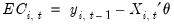 | (55.2) |
Note that it is assumed that both the dependent variable and the regressors have the same number of lags in each cross-section. For notational convenience, it is also assumed that the regressors

, have the same number of lags

in each cross-section, but this assumption is not strictly required for estimation.
PSS derive the concentrated (with respect to the long-run coefficients,

, and the adjustment coefficients,

) log-likelihood function:
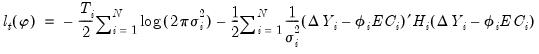 | (55.3) |
where
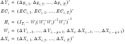 | (55.4) |
where, with some abuse of notation, we define the
j-th lags of

and

as

and

, respectively.
This log-likelihood can be maximized directly. However, PSS suggest an iterative procedure based upon the first derivatives of (2). Initial least squares estimates of

based on the regression

(where

and

are the stacked forms of

and

) are used to compute estimates, using the first-derivative relationships, of

and

. These estimates are then used to compute new estimates of

, and the process continues until convergence. Given the final estimates of

,

and

, estimates of

and

may be computed.
Although this iterative procedure's estimates converge to the full likelihood estimates, their covariance matrix does not. Fortunately, PSS (equation 13, page 625) provide the analytical form of the estimate of the covariance matrix based upon the coefficient estimates.
Estimating PMG Models in EViews
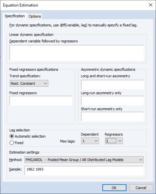
To estimate a Panel ARDL/PMG model in EViews, open the equation dialog by selecting , or by selecting and selecting PMG/ARDL from the Method dropdown menu. EViews will then display the ARDL estimation dialog:
The first tab of the dialog, the Specification tab, allows you to specify the variables used in the regression, and whether to let EViews automatically detect the number of lags for each variable. Enter the dependent variable, followed by a space delimited list of dynamic regressors (i.e. regressors which will have lag terms in the model) in the Dynamic Specification edit box. You may then select whether you wish EViews to automatically select the number of lags for each variable, or whether the number of lags is fixed, using the Automatic Selection and Fixed radio buttons.
If you choose automatic selection, you must then select the maximum number of lags to test for the dependent variable and regressors using the Max lags dropdown menu. If you select to use a fixed number of lags, the same menu may be used to select the number of lags for the dependent variable and regressors. Note that, unlike the non-panel form of ARDL model selection in EViews, each regressor will be given the same number of lags even when using automatic model selection.
The Fixed regressors area lets you specify any fixed/static variables (regressors without lags). The Trend specification dropdown may be used to specify whether the model includes a constant term, or a constant and trend, or neither. Finally, any other static regressors should be entered in the List of fixed regressors box.
The Options tab of the dialog lets you specify the type of model selection to be used if you chose automatic selection on the Specification tab. You may choose between the Akaike Information Criterion (AIC), Schwarz Criterion (SC), or Hannan-Quinn Criterion (HQ) as methods for selection.
Once you have clicked the OK button on the estimation dialog, EViews will present you with the estimation results for both the long-run and short-run coefficients. The presented short-run coefficients (and standard errors) are the mean (and standard deviation) of the cross-section specific coefficients. A separate menu item allows you to see the cross-section specific coefficients in detail.