Descriptive Statistics & Tests
This set of views displays various summary statistics for the series. The submenu contains entries for histograms, basic statistics, and statistics by classification.
Histogram and Stats
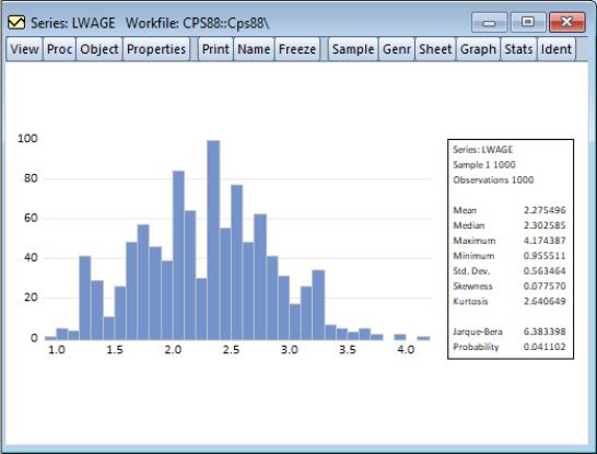
This view displays the frequency distribution of your series in a histogram. The histogram divides the series range (the distance between the maximum and minimum values) into a number of equal length intervals or bins and displays a count of the number of observations that fall into each bin.
(If you would like to produce a histogram where you have greater control over the bin width and placement, or if you would like to construct related graphs such as a kernel density plot or histogram polynomial, you should use the graph view of the series.)
A complement of standard descriptive statistics are displayed along with the histogram. All of the statistics are calculated using the observations in the current sample.
• Mean is the average value of the series, obtained by adding up the series and dividing by the number of observations.
• Median is the middle value (or average of the two middle values) of the series when the values are ordered from the smallest to the largest. The median is a robust measure of the center of the distribution that is less sensitive to outliers than the mean.
• Max and Min are the maximum and minimum values of the series in the current sample.
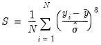
• Std. Dev. (standard deviation) is a measure of dispersion or spread in the series. The standard deviation is given by:
 | (11.1) |
where

is the number of observations in the current sample and

is the mean of the series.
• Skewness is a measure of asymmetry of the distribution of the series around its mean. Skewness is computed as:
 | (11.2) |
where

is an estimator for the standard deviation that is based on the biased estimator for the variance
. The skewness of a symmetric distribution, such as the normal distribution, is zero. Positive skewness means that the distribution has a long right tail and negative skewness implies that the distribution has a long left tail.
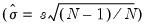
• Kurtosis measures the peakedness or flatness of the distribution of the series. Kurtosis is computed as
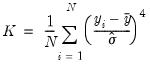 | (11.3) |
where

is again based on the biased estimator for the variance. The kurtosis of the normal distribution is 3. If the kurtosis exceeds 3, the distribution is peaked (leptokurtic) relative to the normal; if the kurtosis is less than 3, the distribution is flat (platykurtic) relative to the normal.
• Jarque-Bera is a test statistic for testing whether the series is normally distributed. The test statistic measures the difference of the skewness and kurtosis of the series with those from the normal distribution. The statistic is computed as:
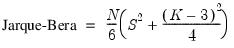 | (11.4) |
where

is the skewness, and

is the kurtosis.
Under the null hypothesis of a normal distribution, the Jarque-Bera statistic is distributed as

with 2 degrees of freedom. The reported Probability is the probability that a Jarque-Bera statistic exceeds (in absolute value) the observed value under the null hypothesis—a small probability value leads to the rejection of the null hypothesis of a normal distribution. For the LWAGE series displayed above, we reject the hypothesis of normal distribution at the 5% level but not at the 1% significance level.
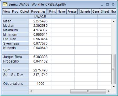
Stats Table
The view displays descriptive statistics for the series in tabular form.
Note that this view provides slightly more information than the view.
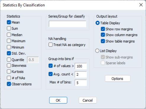
Stats by Classification
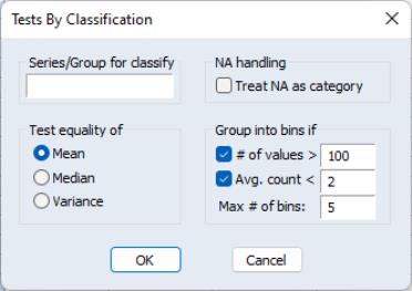
This view allows you to compute the descriptive statistics of a series for various subgroups of your sample. If you select a dialog box appears:
The Statistics option at the left allows you to choose the statistic(s) you wish to compute.
In the
Series/Group for Classify field enter series or group names that define your subgroups. You must type at least one name. Descriptive statistics will be calculated for each unique value of the classification series (also referred to as a factor) unless binning is selected. You may type more than one series or group name; separate each name by a space. The quantile statistic requires an additional argument (a number between 0 and 1) corresponding to the desired quantile value. Click on the button to choose between various methods of computing the quantiles. See
“Empirical CDF” for details.
By default, EViews excludes observations which have missing values for any of the classification series. To treat NA values as a valid subgroup, select the NA handling option.
The Layout option allows you to control the display of the statistics. Table layout arrays the statistics in cells of two-way tables. The list form displays the statistics in a single line for each classification group.
The and options are only relevant if you use more than one series as a classifier.
The Sparse Labels option suppresses repeating labels in list mode to make the display less cluttered.
The Row Margins, Column Margins, and Table Margins instruct EViews to compute statistics for aggregates of your subgroups. For example, if you classify your sample on the basis of gender and age, EViews will compute the statistics for each gender/age combination. If you elect to compute the marginal statistics, EViews will also compute statistics corresponding to each gender, and each age subgroup.
A classification may result in a large number of distinct values with very small cell sizes. By default, EViews automatically groups observations into categories to maintain moderate cell sizes and numbers of categories. Group into Bins provides you with control over this process.
Setting the of values option tells EViews to group data if the classifier series takes more than the specified number of distinct values.
The Avg. count option is used to bin the series if the average count for each distinct value of the classifier series is less than the specified number.
The Max # of bins specifies the maximum number of subgroups to bin the series. Note that this number only provides you with approximate control over the number of bins.
The default setting is to bin the series into 5 subgroups if either the series takes more than 100 distinct values or if the average count is less than 2. If you do not want to bin the series, unmark both options.
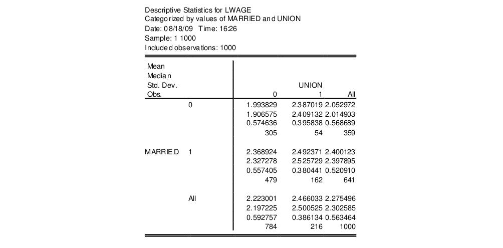
For example, consider the following stats by classification table view of the series LWAGE, categorized by values of MARRIED and UNION (from the workfile “Cps88.WF1”):
The header indicates that the table cells are categorized by two series MARRIED and UNION. These two series are dummy variables that take only two values. No binning is performed; if the series were binned, intervals rather than a number would be displayed in the margins.
The upper left cell of the table indicates the reported statistics in each cell; in this case, the median and the number of observations are reported in each cell. The row and column labeled All correspond to the Row Margin and Column Margin options described above.
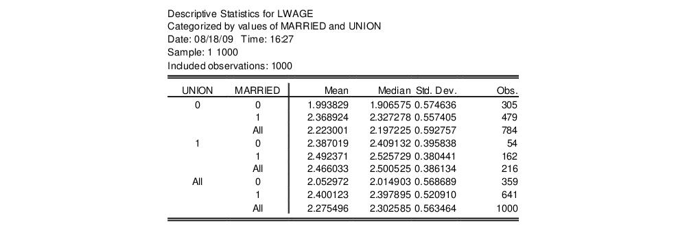
Here is the same view in list form with sparse labels:
For series functions that compute by-group statistics and produce new series, see
“By-Group Statistics”.
Simple Hypothesis Tests
This view carries out simple hypothesis tests regarding the mean, median, and the variance of the series. These are all single sample tests; see
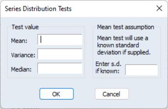
“Equality Tests by Classification” for a description of two sample tests. If you select , the dialog box will be displayed. Depending on which edit field on the left you enter a value, EViews will perform a different test.
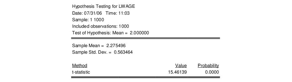
Mean Test
Carries out the test of the null hypothesis that the mean

of the series
X is equal to a specified value

against the two-sided alternative that it is not equal to

:
 | (11.5) |
If you do not specify the standard deviation of X, EViews reports a t-statistic computed as:
 | (11.6) |
where

is the sample mean of X,

is the unbiased sample standard deviation, and

is the number of observations of X. If X is normally distributed, under the null hypothesis the
t-statistic follows a
t-distribution with

degrees of freedom.
If you specify a value for the standard deviation of X, EViews also reports a z-statistic:
 | (11.7) |
where

is the specified standard deviation of
X. If
X is normally distributed with standard deviation

, under the null hypothesis, the
z-statistic has a standard normal distribution.
To carry out the mean test, type in the value of the mean under the null hypothesis in the edit field next to Mean. If you want to compute the z-statistic conditional on a known standard deviation, also type in a value for the standard deviation in the right edit field. You can type in any number or standard EViews expression in the edit fields.
The reported probability value is the p-value, or marginal significance level, against a two-sided alternative. If this probability value is less than the size of the test, say 0.05, we reject the null hypothesis. Here, we strongly reject the null hypothesis for the two-sided test of equality. The probability value for a one-sided alternative is one half the p-value of the two-sided test.
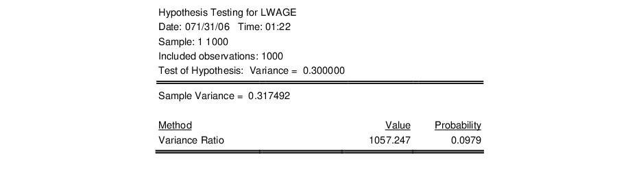
Variance Test
Carries out the test of the null hypothesis that the variance of a series
X is equal to a specified value

against the two-sided alternative that it is not equal to

:
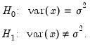 | (11.8) |
EViews reports a

statistic computed as:
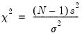 | (11.9) |
where

is the number of observations,

is the sample standard deviation, and

is the sample mean of
X. Under the null hypothesis and the assumption that
X is normally distributed, the statistic follows a

distribution with

degrees of freedom. The probability value is computed as min

, where

is the probability of observing a

-statistic as large as the one actually observed under the null hypothesis.
To carry out the variance test, type in the value of the variance under the null hypothesis in the field box next to Variance. You can type in any positive number or expression in the field.
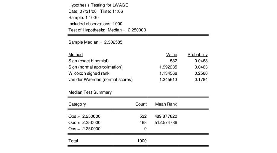
Median Test
Carries out the test of the null hypothesis that the median of a series
X is equal to a specified value

against the two-sided alternative that it is not equal to

:
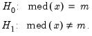 | (11.10) |
EViews reports three rank-based, nonparametric test statistics. The principal references for this material are Conover (1980) and Sheskin (1997).
• Binomial sign test. This test is based on the idea that if the sample is drawn randomly from a binomial distribution, the sample proportion above and below the true median should be one-half. Note that EViews reports two-sided p-values for both the sign test and the large sample normal approximation (with continuity correction).
• Wilcoxon signed ranks test. Suppose that we compute the absolute value of the difference between each observation and the mean, and then rank these observations from high to low. The Wilcoxon test is based on the idea that the sum of the ranks for the samples above and below the median should be similar. EViews reports a p-value for the asymptotic normal approximation to the Wilcoxon T-statistic (correcting for both continuity and ties). See Sheskin (1997, p. 82–94) and Conover (1980, p. 284).
• Van der Waerden (normal scores) test. This test is based on the same general idea as the Wilcoxon test, but is based on smoothed ranks. The signed ranks are smoothed by converting them to quantiles of the normal distribution (normal scores). EViews reports the two-sided p-value for the asymptotic normal test described by Conover (1980).
To carry out the median test, type in the value of the median under the null hypothesis in the edit box next to Median. You can type any numeric expression in the edit field.
Equality Tests by Classification
This view allows you to test equality of the means, medians, and variances across subsamples (or subgroups) of a single series. For example, you can test whether mean income is the same for males and females, or whether the variance of education is related to race. The tests assume that the subsamples are independent.
For single sample tests, see the discussion of
“Simple Hypothesis Tests”. For tests of equality across different series, see
“Tests of Equality”.
Select and the dialog box appears.
First, select whether you wish to test the mean, the median or the variance. Specify the subgroups, the NA handling, and the grouping options as described in
“Stats by Classification”.
Mean Equality Test
This test is a single-factor, between-subjects, analysis of variance (ANOVA). The basic idea is that if the subgroups have the same mean, then the variability between the sample means (between groups) should be the same as the variability within any subgroup (within group).
Denote the
i-th observation in subgroup

as

, where

for groups
. The between and within sums of squares are defined as:
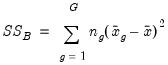 | (11.11) |
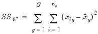 | (11.12) |
where

is the sample mean within group

and

is the overall sample mean. The
F-statistic for the equality of group means is computed as:
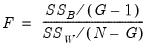 | (11.13) |
where

is the total number of observations. The
F-statistic has an
F-distribution with

numerator degrees of freedom and

denominator degrees of freedom under the null hypothesis of independent and identical normal distributed data, with equal means and variances in each subgroup.
When the subgroup variances are heterogeneous, we may use the Welch (1951) version of the test statistic. The basic idea is to form a modified F-statistic that accounts for the unequal variances. Using the Cochran (1937) weight function,
 | (11.14) |
where

is the sample variance in subgroup

, we form the modified
F-statistic
 | (11.15) |
where

is a normalized weight and

is the weighted grand mean,
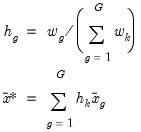 | (11.16) |
The numerator of the adjusted statistic is the weighted between-group mean squares and the denominator is the weighted within-group mean squares. Under the null hypothesis of equal means but possibly unequal variances,

has an approximate
F-distribution with
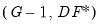
degrees-of-freedom, where
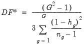 | (11.17) |
For tests with only two subgroups

, EViews also reports the
t-statistic, which is simply the square root of the
F-statistic with one numerator degree of freedom. Note that for two groups, the Welch test reduces to the Satterthwaite (1946) test.
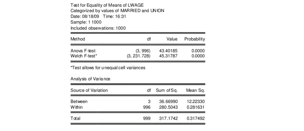
The top portion of the output contains the ANOVA results for a test of equality of means for LWAGE categorized by the four groups defined by the series MARRIED and UNION:
The results show that there is strong evidence that LWAGE differs across groups defined by MARRIED and UNION; both the standard ANOVA and the Welch adjusted ANOVA statistics are in excess of 40, with probability values near zero.
The analysis of variance table shows the decomposition of the total sum of squares into the between and within sum of squares, where:
Mean Sq. = Sum of Sq./df
The F-statistic is the ratio:
F = Between Mean Sq./Within Mean Sq.
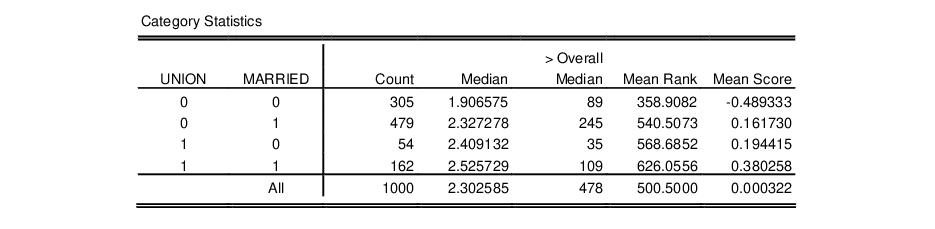
The bottom portion of the output provides the category statistics:
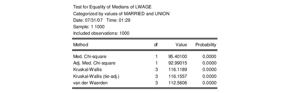
Median (Distribution) Equality Tests
EViews computes various rank-based nonparametric tests of the hypothesis that the subgroups have the same general distribution, against the alternative that at least one subgroup has a different distribution.
We note that the “median” category in which we place these tests is somewhat misleading since the tests focus more generally on the equality of various statistics computed across subgroups. For example, the Wilcoxon test examines the comparability of mean ranks across subgroups. The categorization reflects common usage for these tests and various textbook definitions. The tests should, of course, have power against median differences.
In the two group setting, the null hypothesis is that the two subgroups are independent samples from the same general distribution. The alternative hypothesis may loosely be defined as “the values [of the first group] tend to differ from the values [of the second group]” (see Conover 1980, p. 281 for discussion). See also Bergmann, Ludbrook and Spooren (2000) for a more precise analysis of the issues involved.
• Wilcoxon rank sum test. This test is computed when there are two subgroups. The test is identical to the Wilcoxon signed rank median test (
“Median Test”) but the division of the series into two groups is based upon the values of the classification variable instead of the value of the observation relative to the median.
• Chi-square test for the median. This is a rank-based ANOVA test based on the comparison of the number of observations above and below the overall median in each subgroup. This test is sometimes referred to as the median test (Conover, 1980).
Under the null hypothesis, the median chi-square statistic is asymptotically distributed as a

with

degrees of freedom. EViews also reports Yates’ continuity corrected statistic. You should note that the use of this correction is controversial (Sheskin, 1997, p. 218).
• Kruskal-Wallis one-way ANOVA by ranks. This is a generalization of the Mann-Whitney test to more than two subgroups. The idea behind the Mann-Whitney test is to rank the series from smallest value (rank 1) to largest, and to compare the sum of the ranks from subgroup 1 to the sum of the ranks from subgroup 2. If the groups have the same median, the values should be similar.
EViews reports the asymptotic normal approximation to the U-statistic (with continuity and tie correction) and the
p-values for a two-sided test. For details, see Sheskin (1997). The test is based on a one-way analysis of variance using only ranks of the data. EViews reports the

chi-square approximation to the Kruskal-Wallis test statistic (with tie correction). Under the null hypothesis, this statistic is approximately distributed as a

with

degrees of freedom (see Sheskin, 1997).
• van der Waerden (normal scores) test. This test is analogous to the Kruskal-Wallis test, except that we smooth the ranks by converting them into normal quantiles (Conover, 1980). EViews reports a statistic which is approximately distributed as a

with

degrees of freedom under the null hypothesis.
The top portion of the output displays the test statistics:
In addition to the test statistics and p-values, EViews reports values for the components of the test statistics for each subgroup of the sample. For example, the column labeled Mean Score contains the mean values of the van der Waerden scores (the smoothed ranks) for each subgroup.
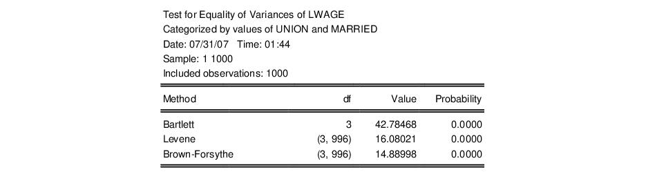
Variance Equality Tests
Variance equality tests evaluate the null hypothesis that the variances in all

subgroups are equal against the alternative that at least one subgroup has a different variance. See Conover,
et al. (1981) for a general discussion of variance equality testing.
• F. This test statistic is reported only for tests with two subgroups

. First, compute the variance for each subgroup and denote the subgroup with the larger variance as

and the subgroup with the smaller variance as

. Then the
F-statistic is given by:
 | (11.18) |
where

is the variance in subgroup

. This
F-statistic has an
F-distribution with

numerator degrees of freedom and

denominator degrees of freedom under the null hypothesis of equal variance and independent normal samples.
• Siegel-Tukey test. This test statistic is reported only for tests with two subgroups

. The test assumes the two subgroups are independent and have equal medians. The test statistic is computed using the same steps as the Kruskal-Wallis test described above for the median equality tests (
“Median (Distribution) Equality Tests”), with a different assignment of ranks. The ranking for the Siegel-Tukey test alternates from the lowest to the highest value for every other rank. The Siegel-Tukey test first orders all observations from lowest to highest. Next, assign rank 1 to the lowest value, rank 2 to the
highest value, rank 3 to the second highest value, rank 4 to the second lowest value, rank 5 to the third lowest value, and so on. EViews reports the normal approximation to the Siegel-Tukey statistic with a continuity correction (Sheskin, 1997, p. 196–207).
• Bartlett test. This test compares the logarithm of the weighted average variance with the weighted sum of the logarithms of the variances. Under the joint null hypothesis that the subgroup variances are equal and that the sample is normally distributed, the test statistic is approximately distributed as a

with

degrees of freedom. Note, however, that the joint hypothesis implies that this test is sensitive to departures from normality. EViews reports the adjusted Bartlett statistic. For details, see Sokal and Rohlf (1995) and Judge,
et al. (1985).
• Levene test. This test is based on an analysis of variance (ANOVA) of the absolute difference from the mean. The
F-statistic for the Levene test has an approximate
F-distribution with

numerator degrees of freedom and

denominator degrees of freedom under the null hypothesis of equal variances in each subgroup (Levene, 1960).
• Brown-Forsythe (modified Levene) test. This is a modification of the Levene test in which we replace the absolute mean difference with the absolute median difference. The Brown-Forsythe test appears to be a superior in terms of robustness and power to Levene (Conover, et al. (1981), Brown and Forsythe (1974a, 1974b), Neter, et al. (1996)).
As with the other equality tests, the top portion of the output displays the test results:
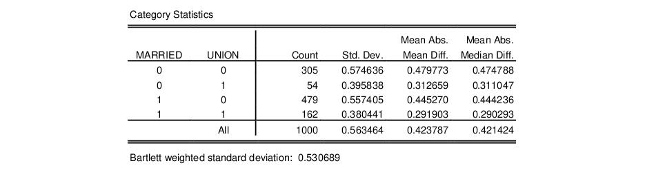
The bottom portion of the output shows the intermediate calculations used in forming the test statistic:
Empirical Distribution Tests
EViews provides built-in Kolmogorov-Smirnov, Lilliefors, Cramer-von Mises, Anderson-Darling, and Watson empirical distribution tests. These tests are based on the comparison between the empirical distribution and the specified theoretical distribution function. For a general description of empirical distribution function testing, see D’Agostino and Stephens (1986).
You can test whether your series is normally distributed, or whether it comes from, among others, an exponential, extreme value, logistic, chi-square, Weibull, or gamma distribution. You may provide parameters for the distribution, or EViews will estimate the parameters for you.
To carry out the test, simply double click on the series and select from the series window.
There are two tabs in the dialog. The tab allows you to specify the parametric distribution against which you want to test the empirical distribution of the series. Simply select the distribution of interest from the drop-down menu. The small display window will change to show you the parameterization of the specified distribution.
You can specify the values of any known parameters in the edit field or fields. If you leave any field blank, EViews will estimate the corresponding parameter using the data contained in the series.
The tab provides control over any iterative estimation that is required. You should not need to use this tab unless the output indicates failure in the estimation process. Most of the options in this tab should be self-explanatory. If you select , EViews will take the starting values from the C coefficient vector.
It is worth noting that some distributions have positive probability on a restricted domain. If the series data take values outside this domain, EViews will report an out-of-range error. Similarly, some of the distributions have restrictions on domain of the parameter values. If you specify a parameter value that does not satisfy this restriction, EViews will report an error message.
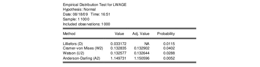
The output from this view consists of two parts. The first part displays the test statistics and associated probability values.
Here, we show the output from a test for normality where both the mean and the variance are estimated from the series data. The first column, “Value”, reports the asymptotic test statistics while the second column, “Adj. Value”, reports test statistics that have a finite sample correction or adjusted for parameter uncertainty (in case the parameters are estimated). The third column reports p-value for the adjusted statistics.
All of the reported EViews p-values will account for the fact that parameters in the distribution have been estimated. In cases where estimation of parameters is involved, the distributions of the goodness-of-fit statistics are non-standard and distribution dependent, so that EViews may report a subset of tests and/or only a range of p-value. In this case, for example, EViews reports the Lilliefors test statistic instead of the Kolmogorov statistic since the parameters of the normal have been estimated. Details on the computation of the test statistics and the associated p-values may be found in Anderson and Darling (1952, 1954), Lewis (1961), Durbin (1970), Dallal and Wilkinson (1986), Davis and Stephens (1989), Csörgö and Faraway (1996) and Stephens (1986).
The second part of the output table displays the parameter values used to compute the theoretical distribution function. Any parameters that are specified to estimate are estimated by maximum likelihood (for the normal distribution, the ML estimate of the standard deviation is subsequently degree of freedom corrected if the mean is not specified a priori). For parameters that do not have a closed form analytic solution, the likelihood function is maximized using analytic first and second derivatives. These estimated parameters are reported with a standard error and p-value based on the asymptotic normal distribution.