Impulse Response Confidence Intervals
In addition to estimating the impulse response path, we may wish to obtain confidence intervals for those estimates. There are a variety of approaches to obtaining these estimates.
Analytic Asymptotic (Delta Method)
An extensive theoretical overview on analytic confidence intervals may be found in Chapter 3 of Lütkepohl (2005).
Briefly, the theoretical results are based on a first-order expansion (delta method) of the asymptotic normal distribution of the impulse response estimate.
Without loss of generality (
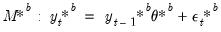
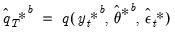
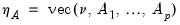
i.e., remaining agnostic about the method of estimation and structural identification), consider an arbitrary full impulse response path

matrix:
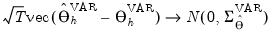
and let
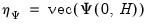
and
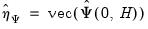
denote respectively the vectorized forms of

and its estimate. Then, as usual, we have the following asymptotic result:
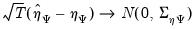 | (46.20) |
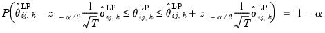
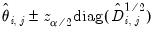
Then, as usual, we can construct confidence interval bands for the impulse response path as:
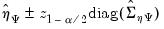 | (46.21) |
where

denotes the

-vector of diagonal elements of the estimated covariance matrix

, and

denotes the

-quantile of the standard Gaussian distribution.
Note that these bands capture the unconditional uncertainty of the impulse response coefficients at each horizon step

. While these results are both useful and valid, this approach to confidence interval computation ignores the collinearity among impulse response coefficients, and ignores the temporal ordering of the impulse response path. The latter is a particularly important omission as a given value of the impulse response path affects the future trajectory of the path, but not conversely.
Traditional VAR Analytic
Lütkepohl describes analytic estimation of the covariance matrix

for results obtained from traditional VAR estimation and provides the necessary equations for its computation.
Let
and
. Then we have the following asymptotic results:
 | (46.22) |
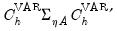
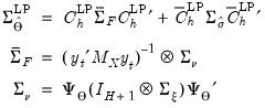
where
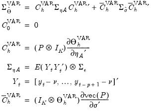 | (46.23) |
and
.
The covariance of the impulse responses,

, described in
Equation (46.23) is the sum of two components:
• 
reflects the uncertainty associated with the slope parameter estimates
• 
captures the uncertainty associated with the estimate of

The nominal

% confidence interval for a specific impulse response coefficient at horizon step

satisfies:
 | (46.24) |
where

is the
-th element of

.
Local Projection Analytic
Sequential Estimation
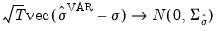
The limiting distribution theory for the sequential local projection impulse response estimator can be derived analogously. Consider again the asymptotic result:
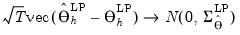 | (46.25) |
where,
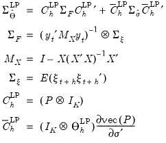 | (46.26) |
where

is the covariance of the

.
 | (46.27) |
where

is the

-th element of

.
Jordà (2005) warns that the innovation process

of the local-projection regression has a moving average component of order

. Although the presence of the moving average doesn’t affect estimator consistency, Jordà (2005) recommends the use of a Newey-West estimator for

at each horizon step

to improve the accuracy of the confidence interval estimate.
Joint Estimation
Since the residuals from a local-projection regression exhibit a moving average component of order

, for sequential estimation, Jordà (2005) recommends use of a Newey-West estimator of the residual covariance matrix at each horizon step

.
Alternately, Jordà (2009), shows it is possible to address this issue parametrically, and derives the correct covariance matrix of the full path of the impulse response coefficients:
 | (46.28) |
where we replace the estimated

in
Equation (46.26) with

, and

is a transformation matrix that depends on the lag coefficients of the LP (Jordà 2009, p. 642).
Recall that the sequential confidence intervals in
Equation (46.24) and
Equation (46.27) ignore collinearity among impulse response coefficients, and the temporal ordering of the impulse response path. To address these issues, Jordà (2009) proposes two simultaneous confidence band computations, the Scheffé band and the conditional error band.
The Scheffé's band is given by:
 | (46.29) |
which we obtain using the LDL decomposition of

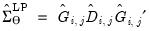 | (46.30) |
where

is a lower triangular matrix with 1’s along the main diagonal;

is a diagonal matrix, and

is the

critical value of

.
An alternative joint confidence band is the conditional error band:
 | (46.31) |
Scheffé bands provide a rectangular approximation to the elliptical simultaneous confidence region of impulse response coefficients. Alternately, conditional error bands separate the variation of each impulse response coefficient from the variation resulting from impulse response serial correlation. Thus, conditional error bands are better at identifying the significance of individual impulse response coefficients analogous to the way a Wald test on coefficient joint significance works.
Note that, even with joint estimation, we can compute the classical confidence bands by ignoring serial correlation and collinearity by deriving the band using only the diagonal elements of

.
Monte Carlo (MC Integration)
An alternative method of computing impulse response confidence intervals is provided by Sims and Zha (1999). This Bayesian approach simulates the posterior distribution of the impulse response conditional on the p pre-sample observations. Assuming Gaussian innovations, the distribution of interest is normal-inverse Wishart. As the theory has only been developed given traditional VAR estimation, we only employ this method in that context.
From
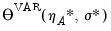
“Impulse Response Confidence Intervals” we see that the impulse response path is a nonlinear function of the vectorized VAR coefficients

, and the vectorized residual covariance matrix

, which we may denote as
The method of MC integration is based on drawing from the posterior distribution,
, where:
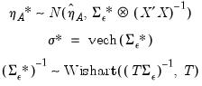 | (46.32) |
The error bands are obtained as the

and

percentiles of the simulated posterior distribution of the impulse response coefficients. Extending the result to structural shocks is straightforward and only requires scaling by an appropriate

.
Bootstrapping
Bootstrap Theory
Suppose there exists a data generating process (DGP) we're interested in estimating. Without loss of generality, we can assume such a DGP is parametric with a particular model specification

, an associated core dataset

, some parameter space

, and an auxiliary data/parameter space

to complete the specification. We can succinctly describe such a DGP as a tuple
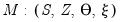 | (46.33) |
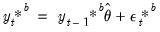
To formalize matters, assume a simple autoregressive DGP of the form
 | (46.34) |
Finally, let the object of statistical interest (e.g., estimator, test statistic, etc.) be some functional of the data and parameters:
 | (46.35) |
Then, the general principle governing bootstrap methods is that distribution

of

can be approximated by generating a large number, say

, of different outcome paths (
with

) for

, where the superscript

indicates that the object is derived from simulation. In particular, the

outcomes

are obtained by simulating from

(via repeated applications of

) to generate

independent outcomes

of

, and for each such draw, estimate

and compute the corresponding

in the same way

was derived from the original data.

is then estimated as the empirical distribution of

.
Note that the final bootstrap estimator of

, typically denoted as

, is derived as the average of the individual bootstrap estimates

. In other words:
 | (46.36) |
Types of Bootstrap
Four our purposes it is useful to distinguish between two types of bootstrap simulation: residual based boostrap and blocks of blocks bootstrap.
Residual Based Bootstrap
In traditional regression settings, the bootstrap procedure often used to obtain

is the
residual based bootstrap. Assuming a simple autoregressive DGP of the form above, the algorithm is summarized below:
1. Estimate

to derive estimates

and the residual process

.
2. For each

:
a. Randomly draw with replacement from

to obtain bootstrap innovations

.
b. Simulate bootstrap data via
(i.e., recursively).
c. Generate the bootstrap DGP:
 | (46.37) |
d. Estimate

to derive estimates

and

.
e. Obtain a bootstrap estimate of the object of interest as:
 | (46.38) |
Block of Blocks Bootstrap
The
block of blocks bootstrap is a non-parametric method designed to accommodate weakly dependent stationary observations. While there are several implementations of this methodology, each addressing important practical aspects, here we only outline the basic idea. In particular, data is bootstrapped by selecting blocks of length

randomly with replacement from

. Again, assuming a simple autoregressive DGP shown earlier, the algorithm is described below:
1. Define

overlapping blocks of data
of length

. In other words, form a matrix
.
2. For each

:
a. Simulate bootstrap data via
where

. In other words, draw with replacement from the columns of

.
b. Generate the bootstrap DGP:
c. Estimate

to derive estimates

and

.
d. Obtain a bootstrap estimate of the object of interest as:
Double Bootstrap
It is sometimes necessary to obtain bootstrapped versions of bootstrap statistics. For instance, the object of interest may be the distribution

of

. This is typically needed in deriving the variance of a bootstrap statistic. In this case, for each
, the distribution

is approximated by generating a large number, say

, of different outcome paths (

with
) for

, where the superscript

indicates that the object is derived from a second stage bootstrap simulation. In particular, the

outcomes

are obtained by simulating from each first stage bootstrap DGP in exactly the same way that

was simulated from the original DGP.

is estimated as the empirical distribution of
 | (46.39) |
Fast Double Bootstrap
Performing a full double bootstrap algorithm is extremely computationally demanding. A single bootstrap algorithm typically requires the computation of

test statistics -- a single statistic performed on the original data and an additional

statistics obtained in the bootstrap loop. On the other hand, a full double bootstrap requires
statistics, with the additional

statistics computed in the inner loop of the double bootstrap algorithm. For instance, setting

and

, the double bootstrap will require the computation of no less than 499,501 test statistics.
Several attempts have been proposed to reduce this computational burden, among the most popular of which is the
fast double bootstrap (FDB) algorithm of Davidson and MacKinnon (2002) and general iterated variants proposed in Davidson and Trokic (2020). The principle governing the success of these algorithms relies on setting

. For instance, the FDB has proved particularly useful in approximating full double bootstrap algorithms with roughly less than the twice the computational burden of the traditional bootstrap:

to be precise.
Traditional VAR Bootstrap
To derive bootstrap confidence intervals for traditional VAR impulse response paths, let

,

,

denote, respectively, some general impulse response coefficient, estimated using the original data

and the DGP in
Equation (46.1), and the associated bootstrap estimator so that

.
The choice of bootstrap algorithm to derive

is not particularly important. Traditionally, a procedure like the residual bootstrap is widely used for traditional VAR impulse response analysis. While modern approaches do suggest the viability of the block of blocks bootstraping, To follow the original literature, however, EViews offers only the residual bootstrap methods described above (
“Residual Based Bootstrap”) for the case of impulse responses derived via traditional VARs.
Confidence Interval Methods
Let

denote a given significance level so that the confidence interval of interest has coverage

. Then, the following bootstrap confidence intervals have been considered in the impulse response literature. See Lütkepohl (2005) for further details.
Standard Percentile Confidence Interval
The most common bootstrap algorithm for impulse response CIs is based on the percentile confidence interval described in Efron and Tibshirani (1993). The bootstrap CI is derived as:
 | (46.40) |
where

and

are respectively the

and

quantiles of the empirical distribution of

.
Hall's Percentile Confidence Interval
An alternative to the
standard percentile CI is the Hall (1992) confidence interval. The idea behind this contribution is that the distribution of

is asymptotically approximated by the distribution of

. Accordingly, the bootstrap CI is derived as:
 | (46.41) |
where

and

are respectively the

and

quantiles of the empirical distribution of
. See Hall (1986) for details.
Hall's Studentized Confidence Interval
Another possibility is to asymptotically approximate the distribution of the studentized statistic

, formalized as:
 | (46.42) |
with the distribution of the bootstrap studentized statistic:
 | (46.43) |
In this case, the bootstrap CI is derived as:
 | (46.44) |
where

and

are respectively the

and

quantiles of the empirical distribution of

where:
 | (46.45) |
See Hall (1986) for details.
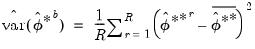
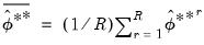
Here,

can be estimated from the

individual bootstrap estimates

. In particular:
 | (46.46) |
where
.
Naturally, extending the argument above,

can be estimated from an additional

double bootstrap estimates

. In this regard, the re-sampling mechanism is obtained by augmenting the residual based bootstrap algorithm to the double bootstrap approach (
“Double Bootstrap”). In particular:
 | (46.47) |
where
.
Alternately, we may employ the less computationally demanding fast double bootstrap approximation. Davidson and Trokic (2020) offer an algorithm to derive confidence intervals based on the FDB. The idea relies on the inverse relationship between

-values and confidence intervals. In particular, any

-value can be converted into a confidence bound through inversion. Thus, the FDB CI algorithm first derives the FDB

-values for a studentized test statistic

that rejects in the lower and upper tails as follows:
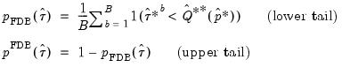 | (46.48) |
where

is the usual indicator function and

is the bootstrap

-value derived as follows:
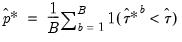 | (46.49) |
and

is the empirical

-quantile of the second stage bootstrap statistics

. Note here that the latter are obtained by setting

, thereby achieving a significant computational speedup.
Next, the algorithm inverts

to obtain the lower and upper confidence bounds by solving the equation:
 | (46.50) |
The solution to this inversion, in case of lower and upper bounds, is as follows:
 | (46.51) |
where

is the empirical

-quantile of the first stage bootstrap statistics

.
Care should be taken however, as Chang and Hall (2015) show that the FDB does not improve asymptotically on the single bootstrap for the construction of confidence intervals.
Kilian's Unbiased Confidence Interval
The Kilian (1998) confidence intervals are specifically designed for VAR impulse response estimates. In particular, this approach explicitly corrects for the bias and skewness in the impulse response estimator that arises due to insufficient observations. We skip over most of the details but an overview of the procedure proceeds as follows:
1. Estimate a VAR to obtain original coefficient estimates.
2. Run a residual bootstrap to obtain bootstrap coefficient estimates which are used to compute a bias correction adjustment to the original estimates.
3. Use the bias corrected coefficients as the basis of a residual double bootstrap to bias correct each of the bootstrap coefficients.
4. Construct the impulse responses using the bias corrected bootstrap coefficients.
5. Derive the

and

empirical quantiles of the bias corrected bootstrap impulse responses.
Note that the nested bootstrap computations required for this method can be costly. A fast bootstrap approximation may be obtained by computing the bias adjustments only once per loop and using it across replications.
Local Projection Bootstrap
One can also rely on bootstrap methods to derive confidence intervals for impulse responses derived via local projections. All that is really necessary is a bootstrap version of the data, namely
, for

. Once generated, we can apply local projection methods outlined in
“Local Projection” in order to estimate

accordingly.
We note here that the literature on bootstrap methods for impulse responses via local projections is not as developed as its traditional VAR counterpart.
While bootstrap methods outlined for traditional VARs are in principle valid for local projection, few papers formally consider the subject of bootstrapping impulse responses computed via local projections. Prominent amongst those that do, Kilian and Kim (2011) argue for using the block of blocks bootstrap to simulate

.
Additional Confidence Interval Methods
In additional to the confidence interval methods describe above in
“Confidence Interval Methods”, we may employ two additional methods specifically designed for use in local projection settings.
Jordà Confidence Interval
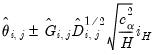
The Jordà (2009) confidence interval is specifically designed for impulse response estimates via local projections. What makes this method unique is that instead of deriving quantiles of impulse response paths directly, it derives quantiles via an auxiliary Wald statistic. We provide an overview of the methodology below:
1. Derive impulse response coefficients via local projections using original data.
2. Derive the Wald statistics below where

is the variance (covariance) of the impulse response coefficient (path):
 | (46.52) |
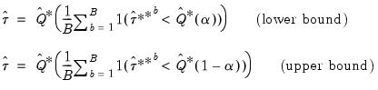
3. Derive the

and

empirical quantiles of

. Let

and

respectively denote the indices associated with these two quantiles.
4. The desired confidence interval is then
 | (46.53) |
Randomized Impulses
Kilian and Kim (2011) offer LP simulation experiments which suggest that treating the impulse matrix as random improves coverage accuracy of intervals compared with those based on initial point estimates for all bootstrap replications.
Traditional VEC Bootstrap
The principles governing the computation of bootstrap CIs for VAR impulse responses remain valid for VEC impulse responses as well. Since every VAR(

) has an equivalent representation as a VEC(

) process, one can simply convert bootstrap VAR estimates into their VEC equivalents, and proceed to derive the VEC impulse responses using the latter coefficients. Alternatively, one can start from a VEC representation, obtain bootstrap coefficient estimates, and then integrate the VEC model to its VAR equivalent. The converted bootstrap coefficient estimates can then be used to derive bootstrap CIs for the corresponding VAR.

 ,
,  , and
, and  .
.