Models
Models Containing Future Endogenous Values
EViews 14 allows you to solve models which contain future values of endogenous variables using standard Gauss-Seidel, and E-Newton or E-QNewton methods (Brayton, 2011).This new capability is central finding solutions to models involving rational expectations.
Consider a model where the equations have the form:
 | (0.5) |
where

is the complete set of equations of the model,

is a vector of all the endogenous variables,

is a vector of all the exogenous variables, and the parentheses follow the usual EViews syntax to indicate leads and lags.
Since solving the model for any particular period requires both past and future values of the endogenous variables, it is not possible to solve the model recursively in one pass. Instead, the equations from all the periods across which the model is to be solved must be treated as a simultaneous system, and solving the model will require terminal as well as initial conditions.
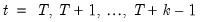
For example, in the case with a single lead and a single lag and a sample that runs from

to

, we must effectively solve the entire stacked system:
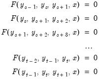 | (0.6) |
where the unknowns are

,

, ...,

the initial conditions are given by

and the terminal conditions are used to determine

. Note that if the leads or lags extend more than one period, we will require multiple periods of initial or terminal conditions.
EViews provides three methods for solving this class of models: Gauss-Seidel, E-Newton, and E-QNewton. All three are iterative procedures that attempt to reduce the change in the endogenous variables,

,

, ...,

, to zero as the model's equations are solved repeatedly.
Gauss-Seidel
The first algorithm, Gauss-Seidel, loops through every observation in the forecast sample and at each observation solves the model while treating the past and future values as fixed. The loop is repeated until changes in the values of the endogenous variables between successive iterations become less than a specified tolerance. In essence, discrepancies between the future value of each endogenous variable and the recalculated value of that variable are diffused forwards and backwards through the observations until the discrepancies vanish, assuming the algorithm converges.
Although the Gauss-Seidel method is not guaranteed to converge, failure to converge is often a sign of model instability which results when the influence of the past or the future on the present does not die out as the length of time considered is increased. Such instability is often undesirable for other reasons and may indicate a poorly specified model.
This method is often referred to as the Fair-Taylor method, although the Fair-Taylor algorithm includes a particular handling of terminal conditions (the extended path method) that is slightly different from the options provided by EViews. When solving the model, EViews allows the user to specify fixed end conditions by providing values for the endogenous variables beyond the end of the forecast sample, or to determine the terminal conditions endogenously by adding extra equations for the terminal periods which impose either a constant level, a linear trend, or a constant growth rate on the endogenous variables for values beyond the end of the forecast period.
E-Newton and E-QNewton
The second and third methods, E-Newton and E-QNewton (
Brayton, 2011), apply the well-known Newton and Broyden methods (respectively) to the problem of finding endogenous variable values such that

. Both algorithms repeatedly construct a linear approximation to the stacked system, use that approximation to adjust the endogenous variables, and update the approximation. These methods involve calculation of the Jacobian of

, or an approximation thereof, and are thus more computationally taxing than Gauss-Seidel.
Weighted against the additional computational cost, these two approaches have the advantage of robustness and applicability to a broader range of models. Small models and those with few future values are frequently solved more efficiently by E-Newton, while large models or those with many future values are solved more efficiently by E-QNewton.
The E-Newton and E-QNewton methods have been implemented as EViews programs and distributed as part of the Federal Reserve's large-scale economic model, FRB/US, in the form of the MCE_SOLVE_LIBRARY. There are a few notable differences between the MCE_SOLVE_LIBRARY and the EViews implementations.
• The MCE_SOLVE_LIBRARY implementation uses a simplifying assumption that future value expressions in the model are strictly linear (option jinit set to "linear"). This option enables Jacobian matrix construction to be performed in a particularly efficient way. However, EViews allows for more general future dependence and currently does not support this feature so that it may take substantially longer to solve this class of linear models.
• The MCE_SOLVE_LIBRARY implementation allows for changing of endogenous variable values at observations outside the solve sample. EViews follows its standard approach and only solves for endogenous variable values at observations within the solve sample.
Forward Solution Options
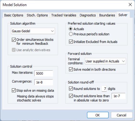
You may click on the button on the model toolbar, or select from the main model object menu to display the solution options.
Click on the tab to display the corresponding dialog page. The dialog page sets options relating to the non-linear equation solver which is applied to the model:
The Solution algorithm box lets you select the algorithm that will be used to solve simultaneous blocks within each period and futures values across all periods (if present). The following choices are available:
• : the Gauss-Seidel algorithm is an iterative algorithm, where at each iteration we solve each equation in the model for the value of its associated endogenous variable, treating all other endogenous variables as fixed.
The Gauss-Seidel algorithm requires little working memory and has fairly low computational costs, but requires the equation system to have certain stability properties for it to converge. Although it is easy to construct models that do not satisfy these properties, in practice, the algorithm generally performs well on most econometric models. If you are having difficulties with the algorithm, you may try reordering the equations, or rewriting the equations to change the assignment of endogenous variables, since these changes can affect the stability of the Gauss-Seidel iterations. (See
“Gauss-Seidel”.)
• : Newton's method is an iterative method, where at each iteration we take a linear approximation to the model, then solve the linear system to find a root of the model.
The Newton algorithm can handle a wider class of problems than Gauss-Seidel, but requires considerably more working memory and has a much greater computational cost when applied to large models. Newton's method is invariant to equation reordering or rewriting. (See
“Newton's Method”.)
• : Broyden's method is a modification of Newton's method (often referred to as a quasi-Newton or secant method) where an approximation to the Jacobian is used when linearizing the model rather than the true Jacobian which is used in Newton's method. This approximation is updated at each iteration by comparing the equation residuals obtained at the new trial values of the endogenous variables with the equation residuals predicted by the linear model based on the current Jacobian approximation.
Because each iteration in Broyden's method is based on less information than in Newton's method, Broyden's method typically requires more iterations to converge to a solution. Since each iteration will generally be cheaper to calculate, however, the total time required for solving a model by Broyden's method will often be less than that required to solve the model by Newton's method.
Note that Broyden's method retains many of the desirable properties of Newton's method, such as being invariant to equation reordering or rewriting. (See
“Broyden's Method”.)
When this method is selected, Broyden's method is used to solve simultaneous blocks but Gauss-Seidel is used to solve future values.
• E-Newton: Simultaneous blocks are solved using Broyden's method and future values are solved using Newton's method.
• E-QNewton: Both simultaneous blocks and future values are solved using Broyden's method.
The Forward solution section allows you to adjust options that affect how the model is solved when one or more equations in the model contain future (forward) values of the endogenous variables.
• The Terminal conditions section lets you specify how the values of the endogenous variables are determined for leads that extend past the end of the forecast period:
If User supplied in Actuals is selected, the values contained in the Actuals series after the end of the forecast sample will be used as fixed terminal values. If no values are available, the solver will be unable to proceed.
If
Constant level is selected, the terminal values are determined endogenously by adding the condition to the model that the values of the endogenous variables are constant over the post-forecast period at the same level as the final forecasted values (

for
), where

is the first observation past the end of the forecast sample, and

is the maximum lead in the model). This option may be a good choice if the model converges to a stationary state.
If Constant difference is selected, the terminal values are determined endogenously by adding the condition that the values of the endogenous variables follow a linear trend over the post forecast period, with a slope given by the difference between the last two forecasted values:
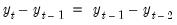 | (0.7) |
for

). This option may be a good choice if the model is in log form and tends to converge to a steady state.
If Constant growth rate is selected, the terminal values are determined endogenously by adding the condition to the model that the endogenous variables grow exponentially over the post-forecast period, with the growth rate given by the growth between the final two forecasted values:
 | (0.8) |
for

).
This latter option may be a good choice if the model tends to produce forecasts for the endogenous variables which converge to constant growth paths.
• The Solve in both directions option affects how the solver loops over periods when calculating forward solutions. When the box is not checked, the solver always proceeds from the beginning to the end of the forecast period during the Gauss-Seidel iterations. When the box is checked, the solver alternates between moving forwards and moving backwards through the forecast period.
The two approaches will generally converge at slightly different rates depending on the level of forward or backward persistence in the model. You should choose whichever setting results in a lower iteration count for your particular model.
Updated command documentation may be found at:
solveopt set solve options for model.
(updated)