ETS Exponential Smoothing in EViews 8
Although ad hoc exponential smoothing (ES) methods have been employed for many decades, recent methodological developments have embedded these models in a modern dynamic nonlinear model framework.
Hyndman, Koehler, et al. (2002, “A State Space Framework For Automatic Forecasting Using Exponential Smoothing Methods,” International Journal of Forecasting, 18, 439–454.) outline the ETS (Error-Trend-Seasonal or ExponenTial Smoothing) framework which defines an extended class of ES methods and offers a theoretical foundation for analysis of these models using state-space based likelihood calculations, with support for model selection and calculation of forecast standard errors.
Notably, the ETS framework encompasses the standard ES models (e.g., Holt and Holt–Winters additive and multiplicative methods), so that it provides a theoretical foundation for what was previously a collection of ad hoc approaches.
EViews 8 provides ETS exponential smoothing as a built-in procedure. Below we show an example of using ETS in EViews.
ETS Smoothing Example
To illustrate estimation and smoothing using an ETS model, we forecast monthly housing starts (HS) for the period 1985m01–1988m12. These data are provided in the workfile hs.wf1.
View a video of this ETS exponential smoothing example.
We will use the multiplicative error, additive trend, and multiplicative seasonal (M, A, M) model to estimate parameters using data from 1959m01–1984m12 and to smooth and forecast for 1985m1–1988m12.
First, load the workfile, open the HS series, and select Proc/Exponential Smoothing/ETS Exponential Smoothing....
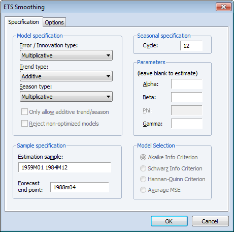
Change the Model specification drop-down menus to (M, A, M), set the Estimation sample to “1959 1984” or “1959m01 1984m12”, set the Forecast end point to “1988m04”, and leave the remaining settings at their default values. When you click OK, EViews estimates the ETS model, displays the results, and saves the smoothed results in the HS_SM series in the workfile.
The results are divided into four parts. The first part of the table shows the settings employed in the ETS procedure, including the sample employed for estimation and the estimation status.
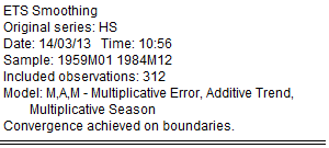
Here we see that we have estimated an (M, A, M) model using data from 1959 to 1984, and that the estimator converged, but with some parameters at boundary values.
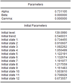
The next section of the table shows the smoothing parameters (α, β, γ)and initial states x0 = (l0, b0, s0, s-1, ..., .s-11). Note the presence of the boundary zero values β for and γ, which indicate that the seasonal and trend components do not change from their initial values.
The bottom portion of the table output contains summary statistics for the estimation procedure:
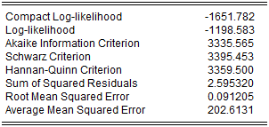
Most of these statistics are self-explanatory. The reported “Compact Log-likelihood” is simply the log-likelihood value absent inessential constants, and is provided to facilitate comparison with results obtained from other sources.
For comparison purposes, it may be useful to consider the ETS model obtained using model selection. To perform model selection, fill out the dialog as before, but set each of the Model specification drop-down menus to Auto.
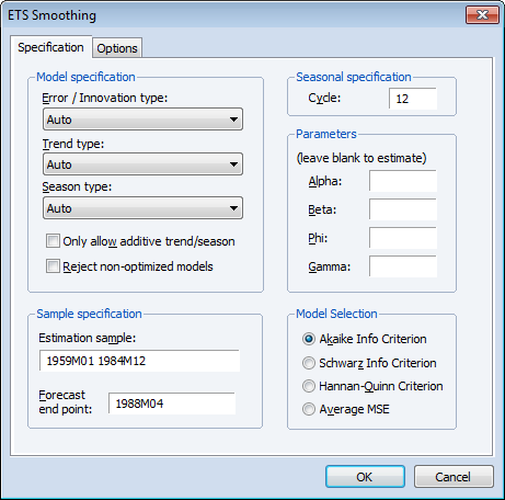
Note that at the default settings, the best model will be selected using the Akaike Information Criterion.
Next, click on the Options tab and set the Display options to show the forecast and all of the elements of the decomposition in Multiple graphs, and to produce graphs and tables for the forecast and likelihood comparisons of all of the models considered by the model selection procedure.
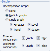
Click on OK to perform the smoothing. Since EViews will be producing several types of output for the procedure, the results will be displayed in a spool:
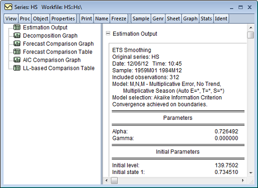
The left output pane allows you to select the output you wish to display. Simply click on the output you wish to display or use the scroll bar on the right side of the window to move from output to output.
The Estimation Output contains the specification, estimated smoothing and initial parameters, and summary statistics. The top portion of the output,
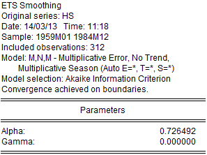
shows that the Akaike information criterion selected ETS model is an (M, N, M) specification, with level smoothing parameter estimate α = 0.72, and the seasonal parameter γ = 0 estimated on the boundary.
The summary statistics indicate that this specification is superior to the earlier (M, A, M) model,
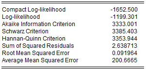
on the basis of all three of the information criteria and the average mean squared error, though the likelihood is lower and the SSR and RMSE are both slightly higher in the selected model.
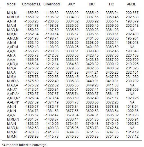
Clicking on the AIC comparison graph in the spool, we see the results for all candidate models:
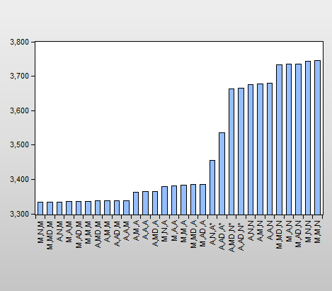
Note that the selected (M, N, M) and the original (M, A, M) model are among the five specifications with relatively low AIC values.
The forecast comparison graph shows the forecasts for the candidate models:
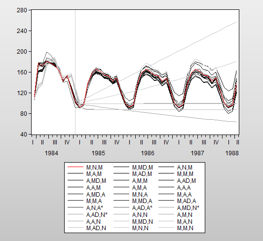
The graph shows both the last few observations of in-sample forecasts and the out-of-sample forecasts for each of the possible ETS specifications.
In addition, our chosen ETS display settings produced both the likelihood table which contains the actual likelihood and Akaike values for each specification, and the forecast comparison table, which presents a subset of the values displayed in the graph. For example, the likelihood table consists of
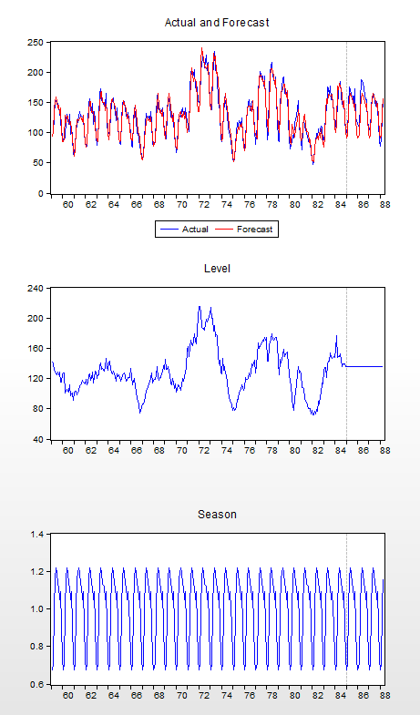
Lastly, the spool contains a multiple graph containing the actual and forecasted values of HS over the estimation and forecast period, along with the decomposition of the series into the level and seasonal components.
