Heckman Selection in EViews 8
The Heckman (1976 “The Common Structure of Statistical Models of Truncation, Sample Selection, and Limited Dependent Variables and a Simple Estimator for Such Models,” Annals of Economic and Social Measurement, 5, 475-492.) selection model, sometimes called the Heckit model, is a method for estimating regression models which suffer from sample selection bias. Under the Heckman selection framework, the dependent variable is only observable for a portion of the data. A classic example, in economics, of the sample selection problem is the wage equation for women, whereby a woman’s wage is only observed if she makes the decision to enter the work place, and is unobservable if she does not. Heckman’s (1976) paper that introduced the Heckman Selection model worked on this very problem.
EViews 8 provides both the Heckman two-step estimator and the maximum likelihood estimator for Heckman selection models.
Below we provide a examples of both Heckman Selection estimation methods.
Heckman's Two Step Estimator Example
View a video of this Heckman Selection Two Step example.
As an example of the estimation of the Heckman Selection model, we take one of the results from Econometric Analysis by William H. Greene (6th Edition, p. 888, Example 24.8), which uses data from the Mroz (1987) study of the labor supply of married women to estimate a wage equation for women. Only 428 of the 753 women studied participated in the labor force, so a selection equation is provided to model the sample selection behavior of married women.
The wage equation is given by:
Wage = β1 + β2Exper + β3Exper2 + β4Educ + β5City + ε
where EXPER is a measure of each woman’s experience, EDUC is her level of education, and CITY is a dummy variable for whether she lives in a city or not.
The selection equation is given by:
LFP = γ1 + γ2Age + γ3Age2 + γ4Faminc + γ5Educ + γ6Kids + υ
where LFP is a binary variable taking a value of 1 if the woman is in the labor force, and 0 otherwise, AGE is her age, FAMINC is the level of household income not earned by the woman, and KIDS is a dummy variable for whether she has children.
You can bring the Mroz data directly into EViews from Greene’s website, using the following EViews command:
wfopen http://www.stern.nyu.edu/~wgreene/Text/Edition7/TableF5- 1.txt
In this data, the wage data are in the series WW, experience is AX, education is in WE, the city dummy is CIT, labor force participation is LFP, age is WA, and family income is FAMINC. There is no kids dummy variable, but there are two variables containing the number of children below K6 education (KL6), and the number of kids between K6 education and 18 (K618). We can create the dummy variable simply by testing whether the sum of those two variables is greater than 0.
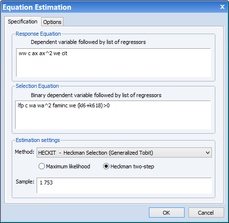
To estimate this equation in EViews, we click on Quick/Estimate Equation…, and then change the equation method to Heckit. In the Response Equation box we type:
ww c ax ax^2 we cit
And in the Selection Equation box we type:
lfp c wa wa^2 faminc we (kl6+k618)>0
We select the Heckman two-step estimation method.

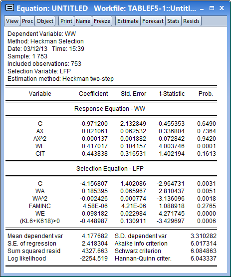
After clicking OK, the estimation results show and replicate the results in the first pane of Table 24.3 in Greene (note that Greene only shows the estimates of the Wage equation).

Maximum Likelihood Example
View a video of this Heckman Selection MLE example.
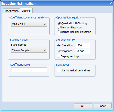
We can modify our equation to use as the estimation method. Click on the Estimate button to bring up the estimation dialog and change the method to Maximum Likelihood. Next, click on the Options tab and change the Coefficient covariance method to OPG - BHHH:

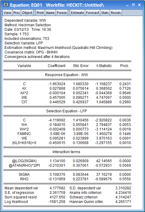
Click on OK to estimate the equation. The results match the second pane of Table 24.3 in Greene.

