Multiple Breakpoint Testing in EViews 8
Tests for parameter instability and structural change in regression models have been an important part of applied econometric work dating back to Chow (1960), who tested for regime change at a priori known dates using an F-statistic. To relax the requirement that the candidate breakdate be known, Quandt (1960) modified the Chow framework to consider the F-statistic with the largest value over all possible breakdates. Andrews (1993) and Andrews and Ploberger (1994) derived the limiting distribution of the Quandt and related test statistics.
More recently, Bai (1997) and Bai and Perron (1998, 2003a) provide theoretical and computational results that further extend the Quandt-Andrews framework by allowing for multiple unknown breakpoints.
EViews 8 introduces these multiple breakpoint tests. Below are some examples of performing the tests in EViews.
Note that these tests are closely related to breakpoint regression.
Least Squares Example
To illustrate the use of these tools in practice, we consider a simple model of the U.S. ex-post real interest rate from Garcia and Perron (1996) that is used as an example by Bai and Perron (2003 “Computation and Analysis of Multiple Structural Change Models,” Journal of Applied Econometrics, 6, 72–78.).
The data, which consist of observations for the three-month treasury rate deflated by the CPI for the period 1961q1–1983q3, are provided in the series RATES in the workfile realrate.wf1. The regression model consists of a constant regressor, and allows for serial correlation that differs across regimes through the use of HAC covariance estimation. We allow up to 5 breaks in the model, and employ a trimming percentage of 15%. Since there are 103 observations in the sample, the trimming value implies that regimes are restricted to have at least 15 observations.
Following Bai and Perron (2003), we begin by estimating the equation specification using least squares. Our equation specification consists of the dependent variable and a single (constant) regressor, so we enter rates c in the specification dialog.
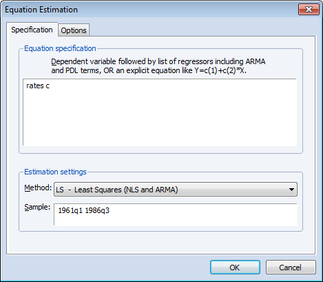
View a video example of this least squares example.
Since we wish to allow for serial correlation in the errors, we specify a quadratic spectral kernel based HAC covariance estimation using prewhitened residuals. The kernel bandwith is determined automatically using the Andrews AR(1) method.
The covariance options may be specified in the Equation Estimation dialog by selecting the Options tab, clicking on the HAC options button and filling out the dialog as shown:
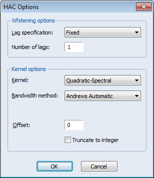
Click on OK to accept the HAC settings, and then on OK to estimate the equation. The estimation results should be as depicted below:
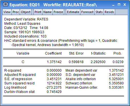
To construct multiple breakpoint tests for this equation, select View/Stability Diagnostics/ Multiple Breakpoint Test... from the equation menu. We consider examples for three different approaches for multiple breakpoint testing with this equation.
Sequential Bai-Perron
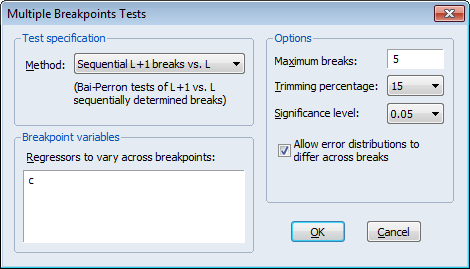
The default Method setting (Sequential L+1 breaks vs. L) instructs EViews to perform sequential testing of l+1 versus l breaks using the methods outlined by Bai (1997) and Bai and Perron (1998).
View a video tutorial of the Bai-Perron Sequential example.
There is a single regressor “C” which we require to be in the list of breaking variables.
By default, the tests allow for a maximum number of 5 breaks, employ a trimming percentage of 15%, and use the 0.05 significance level for the sequential testing. We will leave these options at their default settings. We do, however, select the Allow error distributions to differ across breaks checkbox to allow for error heterogeneity.
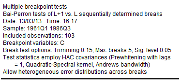
Click on OK to accept the test specification and display the test results. The top portion of the dialog shows the test settings, including the test method, breakpoint variables, test options, and method of computing test covariances. Note that the test employs the same HAC covariance settings used in the original equation but assume regime specific error distributions:
The middle section of the table presents the actual sequential test results:
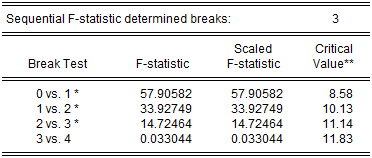
EViews displays the F-statistic, along with the F-statistic scaled by the number of varying regressors (which is the same in this case, since we only have the single, varying regressor), and the Bai-Perron critical value for the scaled statistic. The sequential test results indicate that there are three breakpoints: we reject the nulls of 0, 1, and 2 breakpoints in favor of the alternatives of 1, 2, and 3 breakpoints, but the test of 4 versus 3 breakpoints does not reject the null.
The bottom portion of the output shows the estimated breakdates:

EViews displays both the breakdates obtained from the original sequential procedure, and those obtained following the repartition procedure. In this case, the dates do not change. Again bear in mind that the results follow the EViews convention in defining breakdates to be the first date of the subsequent regime.
Global Bai-Perron L Breaks vs. None
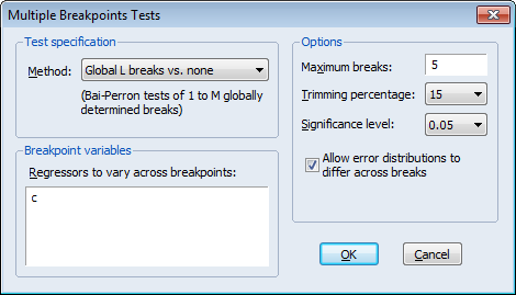
To perform the Bai-Perron tests of l globally optimized breaks against the null of no structural breaks, along with the corresponding UDmax and WDmax tests, simply call up the dialog and change the Method drop-down to Global L breaks vs. none:
View a video tutorial of the Bai-Perron Global L Breaks test.
We again leave the remaining settings at their default values with the exception of the Allow error distributions to differ across breaks checkbox which is selected. Click on OK to perform the test.
The top portion of the output, which shows the test settings, is almost identical to the output for the previous example. The only difference is a line identifying the test method as being “Bai-Perron tests of 1 to M globally determined breaks.”
The middle portion of the output contains the test results:
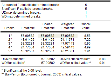
The first four lines summarize the results for different approaches to determining the number of breaks. The “Sequential” result is obtained by performing tests from 1 to the maximum number until we cannot reject the null; the “Significant” result chooses the largest statistically significant breakpoint. In both cases, the multiple breakpoint test indicates that there are 5 breaks. The UDmax and WDmax results show the number of breakpoints as determined by application of the unweighted and weighted maximized statistics. The maximized statistics both indicate the presence of a single break.
The remaining lines show the individual test statistics (original, scaled, weighted) along with the critical values for the scaled statistics. In each case, the statistics far exceed the critical value so that we reject the null of no breaks. Note that the values corresponding to the UDmax and WDmax statistics are shaded for easy identification.
The last two lines of output show the test results for double maximum statistics. In both cases, the maximized value clearly exceeds the critical value, so that we reject the null of no breaks in favor of the alternative of a single break.
The bottom of the portion shows the global optimizers for the breakpoints for each number of breaks:

Note that the three-break global optimizers are the same as those obtained in the sequential testing example. This equivalence will not hold in general.
Global Information Criteria
Lastly, we consider using information criteria to select the number of breaks.
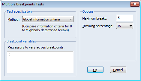
Here we see the dialog when we select Global information criteria in the Method dropdown menu. Note that there are no options for computing the coefficient covariances since this method does not require their calculation. Click on OK to construct the table of results.
The top and bottom portions of the output are similar to the results seen previously so we focus only on the test summaries themselves:
View a video tutorial of the Global Information Critera breakpoint test.
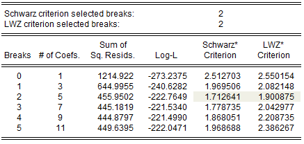
The two summary rows show that both the Schwarz and the LWZ information criteria select 2 breaks. The remainder of the output shows, for each break, the number of estimated coefficients, the optimized sum-of-squared residuals and likelihood, and the values of the information criteria. The minimized Schwarz and LWZ values are shaded for easy identification.
