Panel Cointegration in EViews 8
The analysis of long-run cointegrating relationships has received considerable attention in modern time series analysis. EViews 8 provides new tools for estimating cointegrating relationships using panel data, including various forms of the residual-based panel Fully Modified OLS (FMOLS) and Dynamic OLS (DOLS) estimators (Phillips and Moon, 1999; Pedroni, 2000, 2001; Kao and Chiang, 2000; Mark and Sul, 2003) that produce asymptotically unbiased, normally distributed coefficient estimates.
Below we provide examples of performing panel cointegration estimation in EViews.
Panel Cointegration FMOLS Example
To illustrate the estimation of panel cointegration models in EViews, we follow Kao, Chiang, and Chen (KCC, 1999, “International R&D Spillovers: An Application of Estimation and Inference in Panel Cointegration, Oxford Bulletin of Economics and Statistics, 61, 693–711.) who apply panel cointegration analysis to the study of economic growth by estimating the cointegrating relationship for total factor productivity and domestic and foreign R&D capital stock.
The KCC data, which we provide in the workfile tfpcoint.wf1 consist of annual data on log total factor productivity (LTFP), log domestic (LRD), and log foreign (LFRD) R&D capital stock for 22 countries for the years 1971 to 1990. We consider estimation of simple pooled FMOLS and DOLS estimators for the cointegrating vectors as in Table 4(i) (p. 703) and Table 5(i) (p. 704).
View a video of this FMOLS example.
To begin, display the panel cointegrating equation dialog by clicking on Quick/Estimate Equation... and then selecting COINTREG as the Estimation Method. Note that your workfile must be a panel workfile for the panel cointegration estimation options to be available.
Fill out the top portion of the dialog as depicted below:
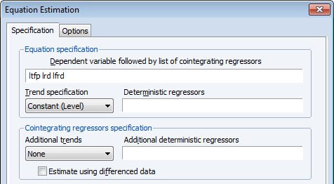
Following KCC, we assume a fixed effect specification with LTFP as the dependent variable and LRD and LFRD as the cointegrating regressors. To handle the fixed effect we specify a Constant (Level) in the Trend specification drop-down menu.
The default panel cointegration estimation method Pooled estimation using Fully-modified OLS (FMOLS) corresponds to the estimates in Table 4(i) of KCC, so we leave those settings unchanged.

To match the KCC estimates, we click on Long-run variances: Options button to display the long-run covariance settings, and change the Kernel options by setting a user-specified bandwidth value of 6:
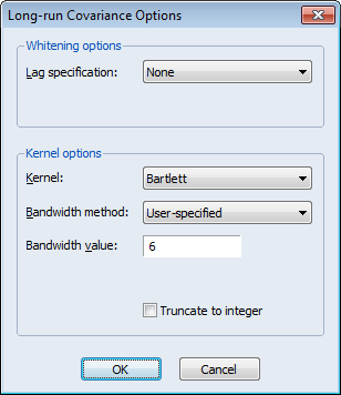
Click on OK to accept the changes. Since we wish to estimate the equation using the default coefficient covariances, we simply click on OK again to estimate the equation using the specified settings. EViews estimates the equation and displays the results:
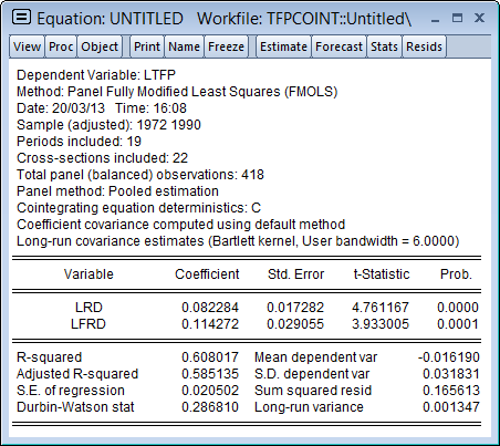
The top portion of the dialog displays the estimation method and information about the sample employed in estimation. Just below the sample information EViews shows that the estimates are based on pooled estimation using only a constant as the cross-section specific trend regressor. The coefficient covariances are computed using the default settings, and the long-run covariances used a Bartlett kernel with the user-specified bandwidth.
The middle section shows the coefficient estimates, standard errors, and t-statistics, which differ a bit from the results in KCC Table 4(i), as KCC report estimates for a slightly different model. As in KCC, both R&D variables, LRD and LFRD are positively related to LTFP, and the coefficients are statistically significant.
The bottom portion of the output shows various summary statistics. Note in particular, the reported “Long-run variance” which shows ω1,2, the estimated long-run average variance of μ1it conditional on μ2it, obtained from the DOLS residuals. The square root of this variance, 0.0367, is somewhat higher than the “S.E. of the regression” value of 0.0205, which is based on the ordinary estimator of the residual variance.
Panel Cointegration DOLS Example
To estimate the model using DOLS, we again display the equation dialog, and fill out the top portion as before:

and change the Method to Dynamic OLS (DOLS). To match the settings in KCC, we set the Panel Method to Pooled, and specify the Fixed lags and leads, with 2 lags and 1 lead:

Click on OK to estimate the equation using the default covariance method. EViews will display the results:
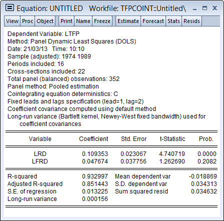
Again, the top portion of the dialog shows the estimation method, sample, and information about settings employed in estimation. Note in particular that the default coefficient covariance matrix computation uses an estimator of the long-run variance computed using a Bartlett kernel and fixed Newey-West bandwidth.
The long-run coefficients, standard errors, and t-statistics are close to their counterparts in KCC Table 5(i).
