Most of the commands that you will employ are object commands. An object command is a command which displays a view of or performs a procedure using a specific object. Object commands have two main parts: an action followed by a view or procedure specification. The (optional) display action determines what is to be done with the output from the view or procedure. The view or procedure specification may provide for options and arguments to modify the default behavior.

The complete syntax for an object command has the form:

where:

There are four possible action commands:

As noted above, in most cases, you need not specify an action explicitly. If no action is specified, the show action is assumed for views and the do action is assumed for most procedures (though some procedures will display newly created output in new windows unless the command was executed via a batch program).

For example, when using an object command to display the line graph series view, EViews implicitly adds a show command. Thus, the following two lines are equivalent:

In this example, the view_or_proc argument is line, indicating that we wish to view a line graph of the GDP data. There are no additional options or arguments specified in the command.

Alternatively, for the equation method (procedure) ls, there is an implicit do action:

so that the two command lines describe equivalent behavior. In this case, the object command will not open the window for EQ1 to display the result. You may display the window by issuing an explicit show command after issuing the initial command:

or by combining the two commands:

Similarly:

both performs the implicit do action and then sends the output to the printer.

The following lines show a variety of object commands with modifiers:

The first example opens a window displaying a line graph of the series GDP. The second example prints (in landscape mode) descriptive statistics for the series in GROUP1. The third example creates a table named OUTPUT1 from the estimation results of EQ1 for a least squares regression of CONS on GDP. The final example executes the forecast procedure of EQ1, putting the forecasted values into the series EQ1F and suppressing any procedure output.

Of these four examples, only the first opens a window and displays output on the screen.

As noted above, the display action determines the destination for view and procedure output. Here we note in passing a few extensions to these general rules.

You may request that a view be simultaneously printed and displayed on your screen by including the letter “p” as an option to the object command. For example, the expression,

is equivalent to the two commands:

since correl is a series view. The “p” option can be combined with other options, separated by commas. So as not to interfere with other option processing, we recommend that the “p” option always be specified after any required options.

Note that the print command accepts the “l” or “p” option to indicate landscape or portrait orientation. For example:

Printer output can be redirected to a text file, frozen output, or a spool object. (See output, and the discussion in “Print Setup” of User’s Guide Ifor details.)

The freeze command used without options creates an untitled graph or table from a view specification:

You also may provide a name for the frozen object in parentheses after the word freeze. For example:

names the frozen bar graph of GDP as “figure1”.

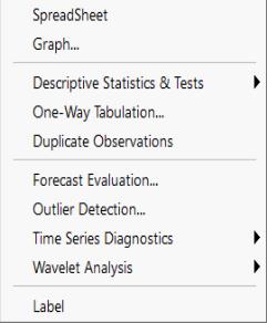
Not surprisingly, the view or procedure commands correspond to elements of the views and procedures menus for the various objects.

For example, the top level of the view menu for the series object allows you to: display a spreadsheet view of the data, graph the data, perform a one-way tabulation, compute and display a correlogram or long-run variance, perform unit root or variance ratio tests, conduct a BDS independence test, or display or modify the label view.

Object commands exist for each of these views. Suppose for example, that you have the series object SER01. Then:

display the spreadsheet and descriptive statistics views of the data in the series. There are a number of graph commands corresponding to the menu entry, so that you may enter:

which display a line graph, bar graph, and histogram, respectively, of the data in SER01. Similarly,

performs a one-way tabulation of the data, and:

display the correlogram and long-run variances, and conduct unit root, variance ratio, and independence testing for the data in the series. Lastly:

appends the text “this is the added series label” to the end of the remarks field.

There are commands for all of the views and procedures of each EViews object. Details on the syntax of each of the object commands may be found in “Object View and Procedure Reference”.