Panel Cointegration Testing
The extensive interest in and the availability of panel data has led to an emphasis on extending various statistical tests to panel data. Recent literature has focused on tests of cointegration in a panel setting. EViews will compute one of the following types of panel cointegration tests: Pedroni (1999), Pedroni (2004), Kao (1999) and a Fisher-type test using an underlying Johansen methodology (Maddala and Wu 1999).
Performing Panel Cointegration Tests in EViews
You may perform a cointegration test using either a Pool object or a Group in a panel workfile setting. We focus here on the panel setting; conducting a cointegration test using a Pool involves only minor differences in specification (see
“Performing Cointegration Tests” for a discussion of testing in the pooled data setting).
To perform the panel cointegration test using a Group object you should first make certain you are in a panel structured workfile (
“Working with Panel Data”). If you have a panel workfile with a single cross-section in the sample, you may perform one of the standard single-equation cointegration tests using your subsample.
Next, open an EViews group containing the series of interest, and select to display the cointegration dialog.
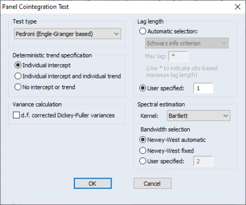
The dropdown menu at the top of the dialog box allow you to choose between three types of tests: Pedroni (Engle-Granger based), Kao (Engle-Granger based), Fisher (combined Johansen). As you select different test types, the remainder of the dialog will change to present you with different options. Here, we see the options associated with the Pedroni test.
(Note, the Pedroni test will only be available for groups containing seven or fewer series.)
The customizable options associated with Pedroni and Kao tests are very similar to the options found in panel unit root testing (
“Cross-sectionally Independent Panel Unit Root Testing”).
The portion of the dialog specifies the exogenous regressors to be included in the second-stage regression. You should select Individual intercept if you wish to include individual fixed effects, Individual intercept and individual trend if you wish to include both individual fixed effects and trends, or No intercept or trend to include no regressors. The Kao test only allows for .
The section is used to determine the number of lags to be included in the second stage regression. If you select EViews will determine the optimum lag using the information criterion specified in the dropdown menu (, , ). In addition you may provide a
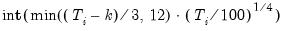
Maximum lag to be used in automatic selection. An empty field will instruct EViews to calculate the maximum lag for each cross-section based on the number of observations. The default maximum lag length for cross-section

is computed as:
where

is the length of the cross-section

. Alternatively, you may provide your own value by selecting
User specified, and entering a value in the edit field.
The Pedroni test employs both parametric and non-parametric kernel estimation of the long run variance. You may use the and sections to control the computation of the parametric variance estimators. The portion of the dialog allows you to specify settings for the non-parametric estimation. You may select from a number of kernel types
(Bartlett, Parzen, Quadratic spectral) and specify how the bandwidth is to be selected (
Newey-West automatic, ,
User specified). The Newey-West fixed bandwidth is given by

. The Kao test uses the and the portion of the dialog settings as described below.
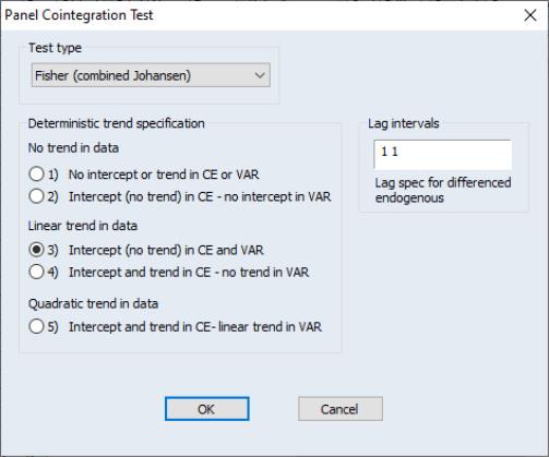
Here, we see the options for the Fisher test selection. These options are similar to the options available in the Johansen cointegration test (
“Johansen Cointegration Test”).
The Deterministic trend specification section determines the type of exogenous trend to be used.
The Lag intervals section specifies the lag-pair to be used in estimation.
Panel Cointegration Details
Here, we provide a brief description of the cointegration tests supported by EViews. The Pedroni and Kao tests are based on Engle-Granger (1987) two-step (residual-based) cointegration tests. The Fisher test is a combined Johansen test.
Pedroni (Engle-Granger based) Cointegration Tests
The Engle-Granger (1987) cointegration test is based on an examination of the residuals of a spurious regression performed using I(1) variables. If the variables are cointegrated then the residuals should be I(0). On the other hand if the variables are not cointegrated then the residuals will be I(1). Pedroni (1999, 2004) and Kao (1999) extend the Engle-Granger framework to tests involving panel data.
Pedroni proposes several tests for cointegration that allow for heterogeneous intercepts and trend coefficients across cross-sections. Consider the following regression
 | (59.5) |
for

;

;
; where

and

are assumed to be integrated of order one,
e.g. I(1). The parameters

and

are individual and trend effects which may be set to zero if desired.
Under the null hypothesis of no cointegration, the residuals

will be I(1). The general approach is to obtain residuals from
Equation (59.5) and then to test whether residuals are I(1) by running the auxiliary regression,
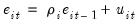 | (59.6) |
or
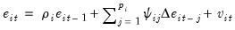 | (59.7) |
for each cross-section. Pedroni describes various methods of constructing statistics for testing for null hypothesis of no cointegration (

). There are two alternative hypotheses: the homogenous alternative,

for all

(which Pedroni terms the within-dimension test or panel statistics test), and the heterogeneous alternative,

for all

(also referred to as the between-dimension or group statistics test).
The Pedroni panel cointegration statistic

is constructed from the residuals from either
Equation (59.6) or
Equation (59.7). A total of eleven statistics with varying degree of properties (size and power for different

and

) are generated.
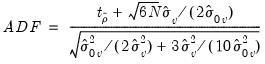
Pedroni shows that the standardized statistic is asymptotically normally distributed,
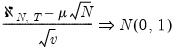 | (59.8) |
where

and

are Monte Carlo generated adjustment terms.
Details for these calculations are provided in the original papers.
Kao (Engle-Granger based) Cointegration Tests
The Kao test follows the same basic approach as the Pedroni tests, but specifies cross-section specific intercepts and homogeneous coefficients on the first-stage regressors.
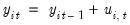
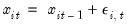
In the bivariate case described in Kao (1999), we have
 | (59.9) |
for
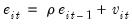
 | (59.10) |
 | (59.11) |
for

;

. More generally, we may consider running the first stage regression
Equation (59.5), requiring the

to be heterogeneous,

to be homogeneous across cross-sections, and setting all of the trend coefficients

to zero.
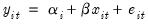
Kao then runs either the pooled auxiliary regression,
 | (59.12) |
or the augmented version of the pooled specification,
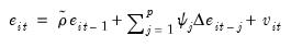 | (59.13) |
Under the null of no cointegration, Kao shows that following the statistics,
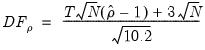 | (59.14) |
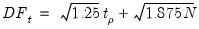 | (59.15) |
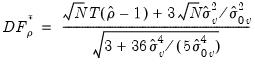 | (59.16) |
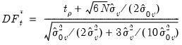 | (59.17) |
and for

(
i.e. the augmented version),
 | (59.18) |
converge to

asymptotically, where the estimated variance is
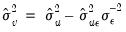
with estimated long run variance
.
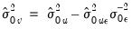
The covariance of
 | (59.19) |
is estimated as
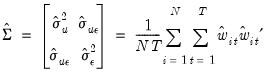 | (59.20) |
and the long run covariance is estimated using the usual kernel estimator
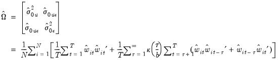 | (59.21) |
where

is one of the supported kernel functions and

is the bandwidth.
Combined Individual Tests (Fisher/Johansen)
Fisher (1932) derives a combined test that uses the results of the individual independent tests. Maddala and Wu (1999) use Fisher’s result to propose an alternative approach to testing for cointegration in panel data by combining tests from individual cross-sections to obtain at test statistic for the full panel.
If

is the
p-value from an individual cointegration test for cross-section

, then under the null hypothesis for the panel,
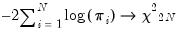 | (59.22) |
By default, EViews reports the

value based on MacKinnon-Haug-Michelis (1999)
p-values for Johansen’s cointegration trace test and maximum eigenvalue test.