EViews Help: Panel Principal Components

In “Panel Covariances”, we discussed how a single panel variable could be unstacked into multiple random variables, allowing us to compute measures of association between different cross-sections or periods. We may extend this basic approach by computing the principal components of the panel variable using one of the measures of association.

The following discussion assumes that you are familiar with the tools for principal components analysis in EViews. Background on the computation, display, and saving of principal components and scores is provided in “Principal Components”.

To compute and display the principal components results for a panel series, open the series, and select View/Panel Principal Components... to display the dialog. Note that the workfile must be structured as a panel for the panel covariance menu entry to be available.

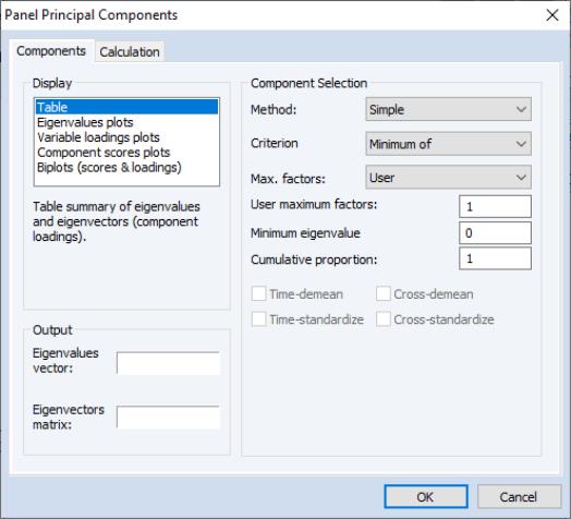
The first tab of the dialog, labeled Components, specifies the display, output, and selection settings for the principal components. The tab is virtually identical to the one displayed when you compute the principal components for a group of series (see “Performing Covariance Analysis”). The one minor difference is in the edit field for the Maximum number of components to be retained. In the panel setting the edit field is filled with “*” which is a stand-in for the maximum number of components (number of cross-sections or periods); in the group setting, this edit field is filled in with the number of variables.

The second tab, labeled Calculation, controls the computation of the measure of association used in the principal components analysis.

Again, the dialog is mostly unchanged from the one used in the group principal components setting with the notable exception of the radio buttons that allow you to choose whether to compute Contemporaneous covariances or Between periods covariances.

The default calculation computes the principal components using the contemporaneous (between cross-section) correlation matrix, but you may use the Type and Method dropdowns choose to use the uncentered Pearson, Spearman rank correlations and Kendall’s tau.

One common task is saving the principal components scores for use in subsequent analysis. Accordingly, EViews provides easy to use tools for saving the scores from your panel principal components analysis in the workfile. As these tools are virtually identical to those documented in “Saving Component Scores”, here, we offer only an abbreviated description.

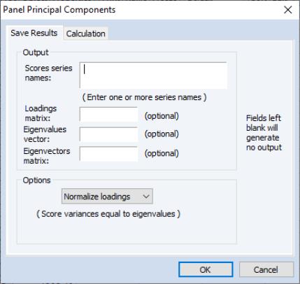
To save the component scores in the workfile, you will use panel principal components procedure. Click on Proc/Make Panel Principal Components... to display the dialog.

The dialog is virtually unchanged from the one displayed for saving principal components scores of a group; indeed the first tab is identical.

In the first tab you will describe the output you wish EViews:

• You should provide names for the series in which you wish to save the scores, and optionally, names for the loadings and eigenvector matrices, and the eigenvalues vector.

• Importantly, the Scaling dropdown on the bottom of the dialog is used to determine the properties of your scores. By default, the scaling is set to Normalize loadings so that the scores have variances equal to the eigenvalues of the decomposition. You may instead elect to save normalized scores (Normalize scores), equal weighted scores and loadings (Symmetric weights), or user weighted loadings (User loading weight).

The second tab is used to describe the computation of the measure of association (used in the computation). The options are those for computing panel covariances as described in “Viewing Principal Components”.

To illustrate, we compute principal components of the cross-country correlations for per capita consumption growth (DCPCH) for the Group of Seven countries over the period from 1973 to 1992 (Obstfeld and Rogoff, 2001). The data, which are from the Penn World Table 5.6, are provided for you in the workfile “PWT56_CONSUMP.wf1” in the Example Files folder in your EViews installation directory.

Open the workfile and the series DCPCH, select View/Panel Principal Components... and click on OK to compute the principal components using the default settings and to display the basic results in table form:

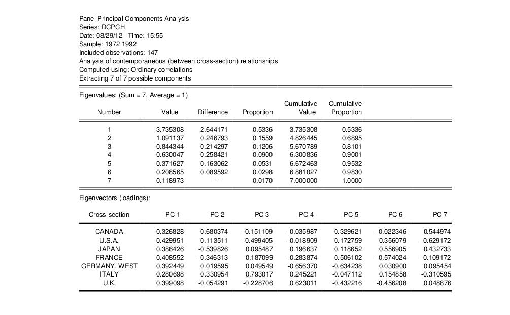
Here we see header information describing the computation and two out of three of the sections of output. The first section provides a summary of the eigenvalues of the correlation matrix, while the second section shows the corresponding eigenvectors. Not depicted here, but present in the actual output, is the estimated correlation matrix itself.

These results in the first section show that the first four components account for about 90% of the total scaled variance in the values of DCPCH between cross-sections. The second section describes the linear combination coefficients. We see that the first principal component (labeled “PC1”) is a roughly-equal linear combination of all seven of the country per capita consumption growth. This component might be thought of as representing the common component in G7 consumption growth.

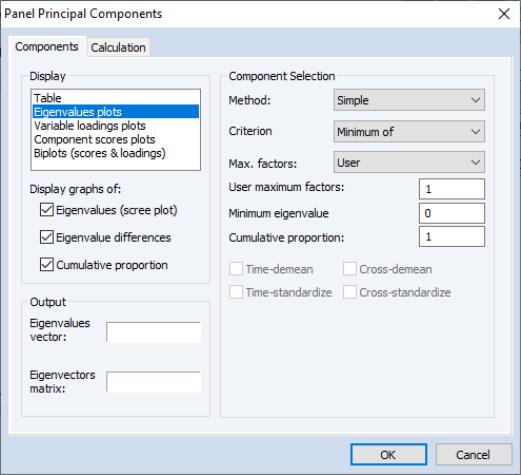
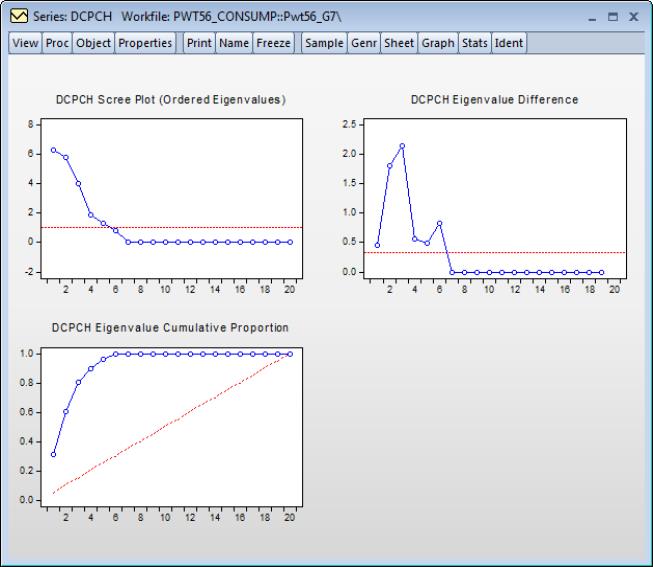
Alternately, we may instruct EViews to compute and graph the eigenvalues associated with the between period correlations. Click on View/Panel Principal Components... to display the dialog

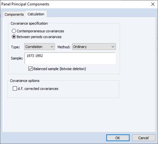
go to the Display section, select Eigenvalues plots and check all of the display checkboxes so that EViews will display all three of the eigenvalue plots. Next, click on the Calculation tab and click on the Between periods covariances button so that EViews will unstack the data into different periods.

It is important to note that you must change the sample to “1973 1992” since data for DCPCH in 1972 are not available (DCPCH is a lagged difference). If you were to use the original sample of “1972 1992”, the balanced sample option would remove all observations and the resulting between period correlation matrix would contain only NAs. Principal components analysis on this matrix would fail.