Residual Diagnostics
EViews provides tests for serial correlation, normality, heteroskedasticity, and autoregressive conditional heteroskedasticity in the residuals from your estimated equation. Not all of these tests are available for every specification.
Correlograms and Q-statistics
This view displays the autocorrelations and partial autocorrelations of the equation residuals up to the specified number of lags. Further details on these statistics and the Ljung-Box
Q-statistics that are also computed are provided in
“Q-Statistics” .
This view is available for the residuals from least squares, two-stage least squares, nonlinear least squares and binary, ordered, censored, and count models. In calculating the probability values for the Q-statistics, the degrees of freedom are adjusted to account for estimated ARMA terms.
To display the correlograms and Q-statistics, push on the equation toolbar. In the dialog box, specify the number of lags you wish to use in computing the correlogram.
Correlograms of Squared Residuals
This view displays the autocorrelations and partial autocorrelations of the squared residuals up to any specified number of lags and computes the Ljung-Box
Q-statistics for the corresponding lags. The correlograms of the squared residuals can be used to check autoregressive conditional heteroskedasticity (ARCH) in the residuals; see also
“ARCH LM Test”, below.
If there is no ARCH in the residuals, the autocorrelations and partial autocorrelations should be zero at all lags and the
Q-statistics should not be significant; see
“Q-Statistics” , for a discussion of the correlograms and
Q-statistics.
This view is available for equations estimated by least squares, two-stage least squares, and nonlinear least squares estimation. In calculating the probability for Q-statistics, the degrees of freedom are adjusted for the inclusion of ARMA terms.
To display the correlograms and Q-statistics of the squared residuals, push on the equation toolbar. In the dialog box that opens, specify the number of lags over which to compute the correlograms.
Histogram and Normality Test
This view displays a histogram and descriptive statistics of the residuals, including the Jarque-Bera statistic for testing normality. If the residuals are normally distributed, the histogram should be bell-shaped and the Jarque-Bera statistic should not be significant; see
“Histogram and Stats” , for a discussion of the Jarque-Bera test.
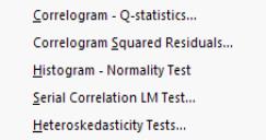
To display the histogram and Jarque-Bera statistic, select. The Jarque-Bera statistic has a

distribution with two degrees of freedom under the null hypothesis of normally distributed errors.
Serial Correlation LM Test
This test is an alternative to the Q-statistics for testing serial correlation. The test belongs to the class of asymptotic (large sample) tests known as Lagrange multiplier (LM) tests.
Unlike the Durbin-Watson statistic for AR(1) errors, the LM test may be used to test for higher order ARMA errors and is applicable whether there are lagged dependent variables or not. Therefore, we recommend its use (in preference to the DW statistic) whenever you are concerned with the possibility that your errors exhibit autocorrelation.
The null hypothesis of the LM test is that there is no serial correlation up to lag order

, where

is a pre-specified integer. The local alternative is ARMA(

) errors, where the number of lag terms

=max(

). Note that this alternative includes both AR(

) and MA(

) error processes, so that the test may have power against a variety of alternative autocorrelation structures. See Godfrey (1988), for further discussion.
The test statistic is computed by an auxiliary regression as follows. First, suppose you have estimated the regression;
 | (26.20) |
where

are the estimated coefficients and

are the errors. The test statistic for lag order

is based on the auxiliary regression for the residuals

:
 | (26.21) |
Following the suggestion by Davidson and MacKinnon (1993), EViews sets any presample values of the residuals to 0. This approach does not affect the asymptotic distribution of the statistic, and Davidson and MacKinnon argue that doing so provides a test statistic which has better finite sample properties than an approach which drops the initial observations.
This is a regression of the residuals on the original regressors

and lagged residuals up to order

. EViews reports two test statistics from this test regression. The
F-statistic is an omitted variable test for the joint significance of all lagged residuals. Because the omitted variables are residuals and not independent variables, the exact finite sample distribution of the
F-statistic under

is still not known, but we present the
F-statistic for comparison purposes.
The Obs*R-squared statistic is the Breusch-Godfrey LM test statistic. This LM statistic is computed as the number of observations, times the (uncentered)

from the test regression. Under quite general conditions, the LM test statistic is asymptotically distributed as a

.
The serial correlation LM test is available for residuals from either least squares or two-stage least squares estimation. The original regression may include AR and MA terms, in which case the test regression will be modified to take account of the ARMA terms. Testing in 2SLS settings involves additional complications, see Wooldridge (1990) for details.
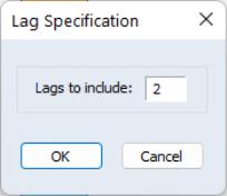
To carry out the test, push on the equation toolbar and specify the highest order of the AR or MA process that might describe the serial correlation. If the test indicates serial correlation in the residuals, LS standard errors are invalid and should not be used for inference.
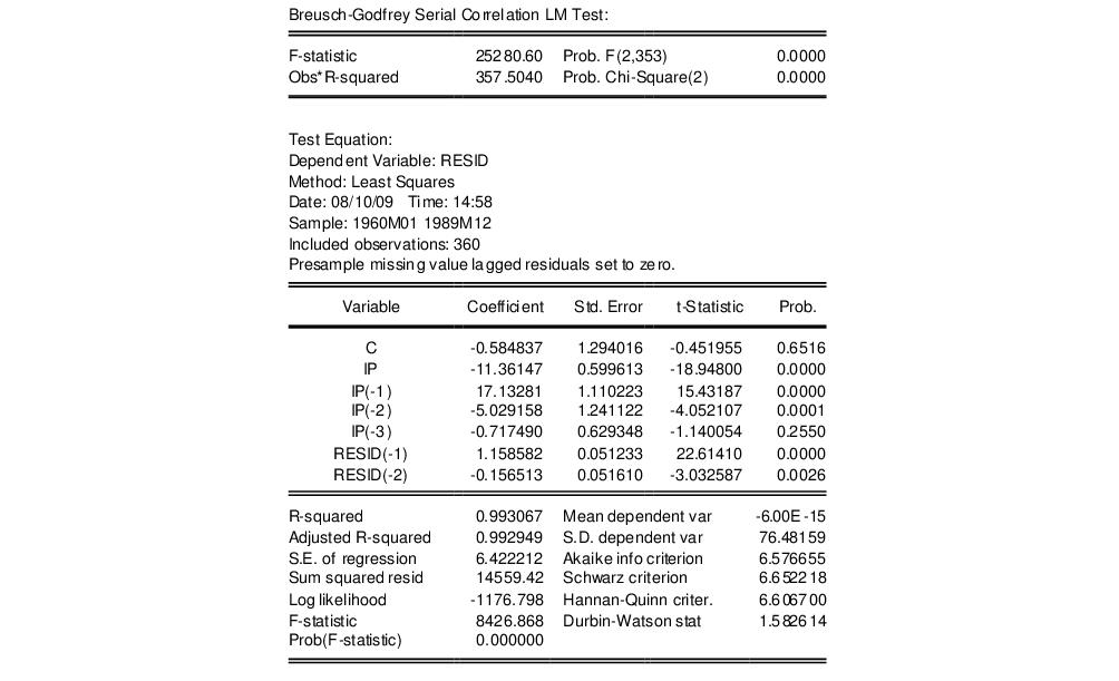
To illustrate, consider the macroeconomic data in our “Basics.WF1” workfile. We begin by regressing money supply M1 on a constant, contemporaneous industrial production IP and three lags of IP using the equation specification
m1 c ip(0 to -3)
The serial correlation LM test results for this equation with 2 lags in the test equation strongly reject the null of no serial correlation:
Heteroskedasticity Tests
This set of tests allows you to test for a range of specifications of heteroskedasticity in the residuals of your equation. Ordinary least squares estimates are consistent in the presence of heteroskedasticity, but the conventional computed standard errors are no longer valid. If you find evidence of heteroskedasticity, you should either choose the robust standard errors option to correct the standard errors (see
“Heteroskedasticity Consistent Covariances”) or you should model the heteroskedasticity to obtain more efficient estimates using weighted least squares.
EViews lets you employ a number of different heteroskedasticity tests, or to use our custom test wizard to test for departures from heteroskedasticity using a combination of methods. Each of these tests involve performing an auxiliary regression using the residuals from the original equation. These tests are available for equations estimated by least squares, two-stage least squares, and nonlinear least squares. The individual tests are outlined below.
Breusch-Pagan-Godfrey (BPG)
The Breusch-Pagan-Godfrey test (see Breusch-Pagan, 1979, and Godfrey, 1978) is a Lagrange multiplier test of the null hypothesis of no heteroskedasticity against heteroskedasticity of the form

, where

is a vector of independent variables. Usually this vector contains the regressors from the original least squares regression, but it is not necessary.
The test is performed by completing an auxiliary regression of the squared residuals from the original equation on

. The explained sum of squares from this auxiliary regression is then divided by

to give an LM statistic, which follows a

-distribution with degrees of freedom equal to the number of variables in

under the null hypothesis of no heteroskedasticity. Koenker (1981) suggested that a more easily computed statistic of Obs*R-squared (where

is from the auxiliary regression) be used. Koenker's statistic is also distributed as a

with degrees of freedom equal to the number of variables in

. Along with these two statistics, EViews also quotes an
F-statistic for a redundant variable test for the joint significance of the variables in

in the auxiliary regression.
As an example of a BPG test suppose we had an original equation of
log(m1) = c(1) + c(2)*log(ip) + c(3)*tb3
and we believed that there was heteroskedasticity in the residuals that depended on a function of LOG(IP) and TB3, then the following auxiliary regression could be performed
resid^2 = c(1) + c(2)*log(ip) + c(3)*tb3
Note that both the ARCH and White tests outlined below can be seen as Breusch-Pagan-Godfrey type tests, since both are auxiliary regressions of the squared residuals on a set of regressors and a constant.
Harvey
The Harvey (1976) test for heteroskedasticity is similar to the Breusch-Pagan-Godfrey test. However Harvey tests a null hypothesis of no heteroskedasticity against heteroskedasticity of the form of

, where, again,

is a vector of independent variables.
To test for this form of heteroskedasticity, an auxiliary regression of the log of the original equation's squared residuals on

is performed. The LM statistic is then the explained sum of squares from the auxiliary regression divided by

, the derivative of the log gamma function evaluated at 0.5. This statistic is distributed as a

with degrees of freedom equal to the number of variables in

. EViews also quotes the Obs*R-squared statistic, and the redundant variable
F-statistic.
Glejser
The Glejser (1969) test is also similar to the Breusch-Pagan-Godfrey test. This test tests against an alternative hypothesis of heteroskedasticity of the form

with

. The auxiliary regression that Glejser proposes regresses the absolute value of the residuals from the original equation upon

. An LM statistic can be formed by dividing the explained sum of squares from this auxiliary regression by

. As with the previous tests, this statistic is distributed from a chi-squared distribution with degrees of freedom equal to the number of variables in

. EViews also quotes the Obs*R-squared statistic, and the redundant variable
F-statistic.
ARCH LM Test
The ARCH test is a Lagrange multiplier (LM) test for autoregressive conditional heteroskedasticity (ARCH) in the residuals (Engle 1982). This particular heteroskedasticity specification was motivated by the observation that in many financial time series, the magnitude of residuals appeared to be related to the magnitude of recent residuals. ARCH in itself does not invalidate standard LS inference. However, ignoring ARCH effects may result in loss of efficiency; see
“ARCH and GARCH Estimation” for a discussion of estimation of ARCH models in EViews.
The ARCH LM test statistic is computed from an auxiliary test regression. To test the null hypothesis that there is no ARCH up to order

in the residuals, we run the regression:
 | (26.22) |
where

is the residual. This is a regression of the squared residuals on a constant and lagged squared residuals up to order

. EViews reports two test statistics from this test regression. The
F-statistic is an omitted variable test for the joint significance of all lagged squared residuals. The Obs*R-squared statistic is Engle’s LM test statistic, computed as the number of observations times the

from the test regression. The exact finite sample distribution of the
F-statistic under

is not known, but the LM test statistic is asymptotically distributed as a

under quite general conditions.
White's Heteroskedasticity Test
White’s (1980) test is a test of the null hypothesis of no heteroskedasticity against heteroskedasticity of unknown, general form. The test statistic is computed by an auxiliary regression, where we regress the squared residuals on all possible (nonredundant) cross products of the regressors. For example, suppose we estimated the following regression:
 | (26.23) |
where the

are the estimated parameters and

the residual. The test statistic is then based on the auxiliary regression:
 | (26.24) |
Prior to EViews 6, White tests always included the level values of the regressors (i.e. the cross product of the regressors and a constant) whether the original regression included a constant term. This is no longer the case—level values are only included if the original regression included a constant.
EViews reports three test statistics from the test regression. The F-statistic is a redundant variable test for the joint significance of all cross products, excluding the constant. It is presented for comparison purposes.
The Obs*R-squared statistic is White’s test statistic, computed as the number of observations times the centered

from the test regression. The exact finite sample distribution of the
F-statistic under

is not known, but White’s test statistic is asymptotically distributed as a

with degrees of freedom equal to the number of slope coefficients (excluding the constant) in the test regression.
The third statistic, an LM statistic, is the explained sum of squares from the auxiliary regression divided by

. This, too, is distributed as chi-squared distribution with degrees of freedom equal to the number of slope coefficients (minus the constant) in the auxiliary regression.
White also describes this approach as a general test for model misspecification, since the null hypothesis underlying the test assumes that the errors are both homoskedastic and independent of the regressors, and that the linear specification of the model is correct. Failure of any one of these conditions could lead to a significant test statistic. Conversely, a non-significant test statistic implies that none of the three conditions is violated.
When there are redundant cross-products, EViews automatically drops them from the test regression. For example, the square of a dummy variable is the dummy variable itself, so EViews drops the squared term to avoid perfect collinearity.
Performing a test for Heteroskedasticity in EViews
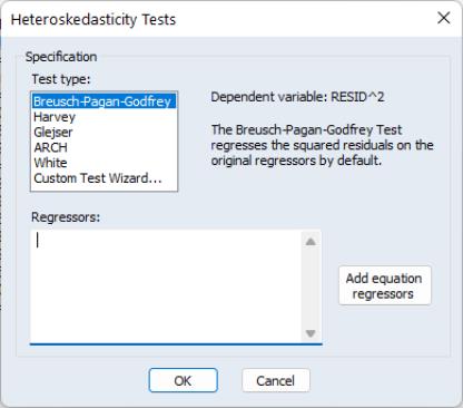
To carry out any of the heteroskedasticity tests, select . This will bring you to the following dialog:
You may choose which type of test to perform by clicking on the name in the box. The remainder of the dialog will change, allowing you to specify various options for the selected test.
The BPG, Harvey and Glejser tests allow you to specify which variables to use in the auxiliary regression. Note that you may choose to add all of the variables used in the original equation by pressing the button. If the original equation was non-linear this button will add the coefficient gradients from that equation. Individual gradients can be added by using the @grad keyword to add the i-th gradient (e.g., “@grad(2)”).
The ARCH test simply lets you specify the number of lags to include for the ARCH specification.
The White test lets you choose whether to include cross terms or no cross terms using the checkbox. The cross terms version of the test is the original version of White's test that includes all of the cross product terms. However, the number of cross-product terms increases with the square of the number of right-hand side variables in the regression; with large numbers of regressors, it may not be practical to include all of these terms. The no cross terms specification runs the test regression using only squares of the regressors.
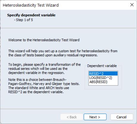
The lets you combine or specify in greater detail the various tests. The following example, using EQ1 from the “Basics.WF1” workfile, shows how to use the Custom Wizard. The equation has the following specification:
log(m1) = c(1) + c(2)*log(ip) + c(3)*tb3
The first page of the wizard allows you to choose which transformation of the residuals you want to use as the dependent variable in the auxiliary regression. Note this is really a choice between doing a Breusch-Pagan-Godfrey, a Harvey, or a Glejser type test. In our example we choose to use the LOG of the squared residuals:
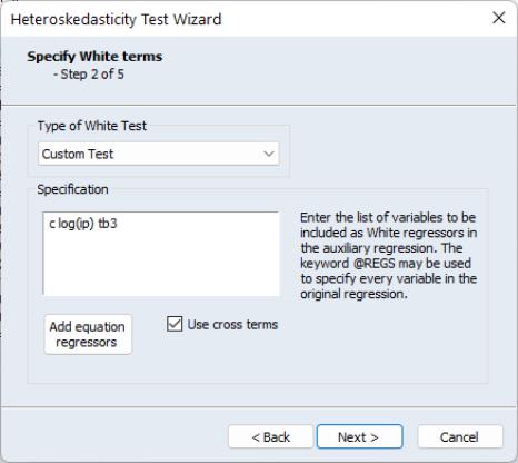
Once you have chosen a dependent variable, click on . Step two of the wizard lets you decide whether to include a White specification. If you check the checkbox and click on Next, EViews will display the page which lets you specify options for the test. If you do not elect to include a White specification and click on , EViews will skip the page, and continue on to the next section of the wizard.
There are two parts to the dialog. In the upper section you may use the Type of White Test dropdown menu to select the basic test.
You may choose to include cross terms or not, whether to run an EViews 5 compatible test (as noted above, the auxiliary regression run by EViews differs slightly in Version 6 and later when there is no constant in the original equation), or, by choosing , whether to include a set of variables not identical to those used in the original equation. The custom test allows you to perform a test where you include the squares and cross products of an arbitrary set of regressors. Note if you when you provide a set of variables that differs from those in the original equation, the test is no longer a White test, but could still be a valid test for heteroskedasticity. For our example we choose to include C and LOG(IP) as regressors, and choose to use cross terms.
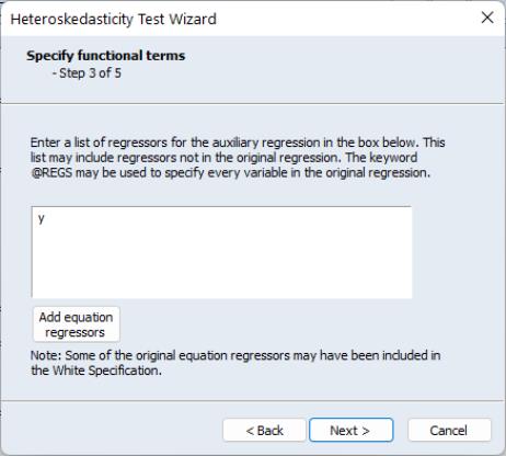
Click on to continue to the next section of the wizard. EViews prompts you for whether you wish to add any other variables as part of a Harvey (Breusch-Pagan-Godfrey/Harvey/Glejser) specification. If you elect to do so, EViews will display a dialog prompting you to add additional regressors. Note that if you have already included a White specification and your original equation had a constant term, your auxiliary regression will already include level values of the original equation regressors (since the cross-product of the constant term and those regressors is their level values). In our example we choose to add the variable Y to the auxiliary regression:
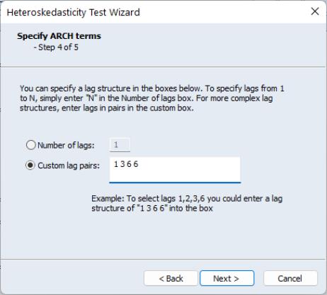
Next we can add ARCH terms to the auxiliary regression. The ARCH specification lets you specify a lag structure. You can either specify a number of lags, so that the auxiliary regression will include lagged values of the squared residuals up to the number you choose, or you may provide a custom lag structure. Custom structures are entered in pairs of lags. In our example we choose to include lags of 1, 2, 3 and 6:
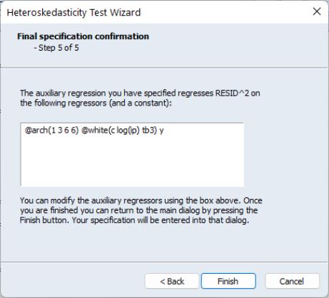
The final step of the wizard is to view the final specification of the auxiliary regression, with all the options you have previously chosen, and make any modifications. For our choices, the final specification looks like this:
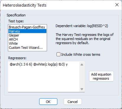
Our ARCH specification with lags of 1, 2, 3, 6 is shown first, followed by the White specification, and then the additional term, Y. Upon clicking Finish the main Heteroskedasticity Tests dialog has been filled out with our specification:
Note, rather than go through the wizard, we could have typed this specification directly into the dialog.
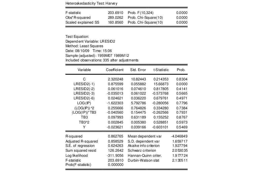
This test results in the following output:
This output contains both the set of test statistics, and the results of the auxiliary regression on which they are based. All three statistics reject the null hypothesis of homoskedasticity.

 distribution with two degrees of freedom under the null hypothesis of normally distributed errors.
 , where
  is a pre-specified integer. The local alternative is ARMA(
 ) errors, where the number of lag terms
  =max(
=max( ). Note that this alternative includes both AR(
 ) and MA(
 ) error processes, so that the test may have power against a variety of alternative autocorrelation structures. See Godfrey (1988), for further discussion.
 are the estimated coefficients and
  are the errors. The test statistic for lag order
  is based on the auxiliary regression for the residuals
  :
:
 and lagged residuals up to order
  . EViews reports two test statistics from this test regression. The F-statistic is an omitted variable test for the joint significance of all lagged residuals. Because the omitted variables are residuals and not independent variables, the exact finite sample distribution of the F-statistic under
  is still not known, but we present the F-statistic for comparison purposes.
 from the test regression. Under quite general conditions, the LM test statistic is asymptotically distributed as a
  .
.
 , where
  is a vector of independent variables. Usually this vector contains the regressors from the original least squares regression, but it is not necessary.
  . The explained sum of squares from this auxiliary regression is then divided by
  to give an LM statistic, which follows a
  -distribution with degrees of freedom equal to the number of variables in
  under the null hypothesis of no heteroskedasticity. Koenker (1981) suggested that a more easily computed statistic of Obs*R-squared (where
  is from the auxiliary regression) be used. Koenker's statistic is also distributed as a
  with degrees of freedom equal to the number of variables in
  . Along with these two statistics, EViews also quotes an F-statistic for a redundant variable test for the joint significance of the variables in
  in the auxiliary regression.
 , where, again,
  is a vector of independent variables.
 is performed. The LM statistic is then the explained sum of squares from the auxiliary regression divided by
  , the derivative of the log gamma function evaluated at 0.5. This statistic is distributed as a
  with degrees of freedom equal to the number of variables in
  . EViews also quotes the Obs*R-squared statistic, and the redundant variable F-statistic.
 with
with  . The auxiliary regression that Glejser proposes regresses the absolute value of the residuals from the original equation upon
  . An LM statistic can be formed by dividing the explained sum of squares from this auxiliary regression by
  . As with the previous tests, this statistic is distributed from a chi-squared distribution with degrees of freedom equal to the number of variables in
  . EViews also quotes the Obs*R-squared statistic, and the redundant variable F-statistic.
 in the residuals, we run the regression:
 is the residual. This is a regression of the squared residuals on a constant and lagged squared residuals up to order
  . EViews reports two test statistics from this test regression. The F-statistic is an omitted variable test for the joint significance of all lagged squared residuals. The Obs*R-squared statistic is Engle’s LM test statistic, computed as the number of observations times the
  from the test regression. The exact finite sample distribution of the F-statistic under
  is not known, but the LM test statistic is asymptotically distributed as a
  under quite general conditions.
 are the estimated parameters and
  the residual. The test statistic is then based on the auxiliary regression:
 from the test regression. The exact finite sample distribution of the F-statistic under
  is not known, but White’s test statistic is asymptotically distributed as a
  with degrees of freedom equal to the number of slope coefficients (excluding the constant) in the test regression.
 . This, too, is distributed as chi-squared distribution with degrees of freedom equal to the number of slope coefficients (minus the constant) in the auxiliary regression.