Impulse Responses Analysis in EViews
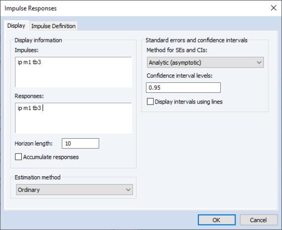
To compute and display impulse responses, click on View/Impulse Response.... on the toolbar of an estimated VAR object to display the dialog interface:
There are sections for Display information, , and Standard errors and confidence intervals on the first tab, settings for Impulse Definition on the second tab, and for Linear projection methods, computational options on a third tab.
Display Information
In the Display tab you will define the Impulses and Responses you initially wish to display, specify the Horizon length over which you wish to compute those impulse responses, and indicate whether to compute cumulative responses using the Accumulate responses checkbox.
Under the Estimation method dropdown, you will specify the method employed to estimate the impulse responses paths. Three choices are available:
• Ordinary - impulse responses are derived via traditional inversion of the estimated VAR coefficients.
• Sequential Local Projection - impulse responses are derived via sequential local projection estimation.
• Joint Local Projection- impulse responses are derived via joint local projection estimation.
In case any of the local projection methods are used, a tab called Local Projection Options appears on the main dialog to allow setting of relevant options.
Note that the Impulses and Responses edit fields are for specifying the initial results to display. By default, these fields are filled out with the names of all of the variables in the VAR, but you will later be able to modify the display interactively. Note also that the impulse occurs in period 1. The default horizon length of 10 displays the period in which the impulse occurs (period 1) and the nine periods that follow.
Standard Errors And Confidence Intervals
The section offer options for the computation of the SEs and the CIs:
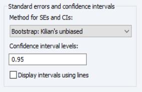
The Method for SEs and CIs dropdown offers several choices:
• None - no SEs and no CIs are produced.
• Monte Carlo - SEs derived by simulating impulses by drawing innovations from the standard normal distribution; CIs computed based on SEs (
“Monte Carlo (MC Integration)”).
• Bootstrap: Jordà's percentile (available only with local projection estimation) - SEs and (traditional) CIs derived using the Jordà (2009) confidence intervals (
“Jordà Confidence Interval”).
• (available only with local projection estimation).
The Confidence intervals levels edit field specifies the intervals to compute. You may provide one or more values in the form of a space delimited list.
By default, EViews uses shading to display CI bands. To use lines instead, check the box next to Display intervals using lines.
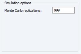
For Monte Carlo and bootstrap-based methods, the Simulation options will show options that control:
• When performing the Monte Carlo procedure, replications are specified in the Monte Carlo replication edit field.
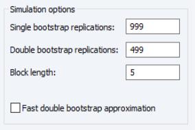
• For bootstrap methods, the section will display a variety of options:
For local projection bootstrap procedures, you will be presented with a Bootstrap DGP method dropdown menu to choose between a based bootstrap or a DGP.
The number of first and possibly second stage bootstrap replications are specified in the corresponding edit fields. Should a full nested double bootstrap be computationally too expensive, you can click on the Fast double bootstrap approximation checkbox.
Impulse Definitions
The Impulse Definition tab provides the following options for specifying the impulses:
• Residual — One Unit: sets the impulses to one unit of the residuals. This option ignores the units of measurement and the correlations in the VAR residuals so that no transformation is performed. The responses from this option are the MA coefficients of the infinite order Wold representation of the VAR.
• Residual—One Std. Dev.: sets the impulses to one standard deviation of the residuals. This option ignores the correlations in the VAR residuals.
• Cholesky: uses the inverse of the Cholesky factor of the residual covariance matrix to orthogonalize the impulses. This option imposes an ordering of the variables in the VAR and attributes all of the effect of any common component to the variable that comes first in the VAR system. Note that responses can change dramatically if you change the ordering of the variables. You may specify a different VAR ordering by reordering the variables in the Cholesky Ordering edit box.
The
(d.f. adjustment) option makes a small sample degrees of freedom correction when estimating the residual covariance matrix used to derive the Cholesky factor. The

-th element of the residual covariance matrix with degrees of freedom correction is computed as
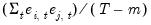
where

is the number of parameters per equation in the VAR. The
(no d.f. adjustment) option estimates the

-th element of the residual covariance matrix as
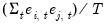
.
• Generalized Impulses: as described by Pesaran and Shin (1998) constructs an orthogonal set of innovations that does not depend on the VAR ordering. The generalized impulse responses from an innovation to the

-th variable are derived by applying a variable specific Cholesky factor computed with the

-th variable at the top of the Cholesky ordering.
• Structural Decomposition: uses the orthogonal transformation estimated from the structural factorization matrices. This approach is not available unless you have estimated the structural factorization matrices as explained in “Structural (Identified) VARs”.
• User Specified allows you to specify your own impulses. Create a matrix (or vector) that contains the impulses and type the name of that matrix in the edit box. If the VAR has

endogenous variables, the impulse matrix must have

rows and 1 or

columns, where each column is an impulse vector.
For example, say you have a

variable VAR and wish to apply simultaneously a positive one unit shock to the first variable and a negative one unit shock to the second variable. Then you will create a vector containing the values 1, -1, and 0. Using commands, you can enter:
vector(3) shock
shock.fill 1,-1,0
and type the name of the vector SHOCK in the edit box.
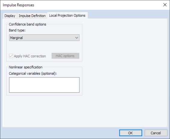
Local Projection Options
If you select Local Projection or Local Projection: Joint under the dropdown menu on the page, the dialog will present you with a tab containing options associated with local projection estimation:
The options will differ slightly for the two local projection methods.
If you select Sequential Local Projection as your , you will see options for correcting for serial correlation when doing estimation.
The
Apply HAC correction should be checked to compute Newey-West, Andrews, or other forms of HAC estimation of the

matrix. Options for the HAC correction can be set by clicking on the
HAC options button.
If you select Joint Local Projectionas your , you will be presented with options for computing different types of confidence interval band types. You may use the Band type dropdown to choose between:
• Marginal - ignores cross-variable and cross-time variation and captures only point-wise impulse response variation.
• Scheffe - captures both cross-variable and cross-time variation and is akin to a rectangular approximation to the elliptical simultaneous confidence region of impulse response coefficients.
• Conditional - captures both cross-variable and cross-time variation which aims to separate the variation of each impulse response coefficient from the variation resulting from impulse response serial correlation.
For both local projection methods, we may perform non-linear local projections (
“Nonlinear Estimation”) as in the regime switching setup of Ahmed and Cassou (2016) by providing a set of optional (space-delimited list of) categorical variables in the
Categorical variables edit box. All of the specified variables will be used to generate a set of dummy variables that span the unique values of the series and are used to generate an impulse response path for each such value.
Displaying Impulse Responses in EViews
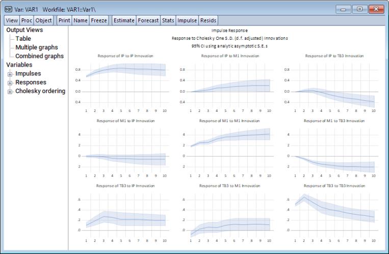
To display the impulse responses, for now, click on OK to accept the default settings and display the impulse responses. Here, EViews displays 9 impulse response graphs including 95% analytic asymptotic confidence bands.
Users may wish to display multiple CI bands. To show 95% and 70% CI bands, for example, enter 0.95 0.7 in the Confidence intervals levels edit field. Doing so yields the following:
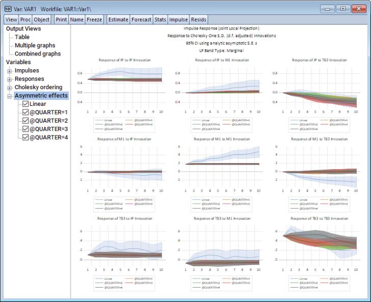
Alternatively, one may wish to study how impulse response paths differ across quarters. To do so, estimate impulse response paths jointly (sequential estimation works as well) by selecting Joint Local Projection from the Estimation method dropdown. Also, click on the Local Projection Options tab and type
@quarter
into the Categorical variables edit field. Finally click on OK. The output is replicated below.
Note that the impulse response output is an interactive spool object with the spool tree listing two collapsible categories (Variables and Output Views) and selectable entries on the left of the window. A category is said to be collapsible when its contents can be collapsed or expanded by clicking on, respectively, the minus or plus box to the left of the category name.
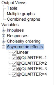
In case nonlinear impulse responses are derived via local projections, a node called Asymmetric effects will become available to allow for toggling the display of each asymmetric effect.
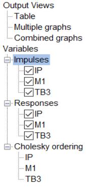
Note further that the Output Views node may be collapsed or expanded to hide or show the three entries which control the type of output displayed:
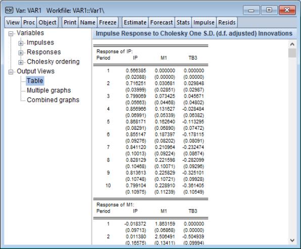
• Table — if selected, will display a table of the impulse response values and standard errors in the right pane.
• Multiple Graphs — if selected, will plot impulse response graphs with one for each requested impulse response combination.
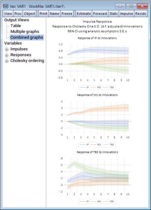
• Combined Graphs — if selected, will plot separate graphs for each requested impulse, with all of the requested responses.
Selecting one of these entries will display the corresponding contents in the right pane of the output window. For example, for an original traditional VAR IR spool output, clicking on the Table entry changes the display show numeric values for the impulse responses and standard errors:
Clicking on the Combined graphs entry yields:
showing the impulse responses in graphs grouped by response variables.
The Variables node may be collapsed or expanded to hide or show the three node entries: Impulses, Responses, and if appropriate, Cholesky ordering.
The Impulses and Responses nodes contain entries for the variables in the VAR with which you may interact to change the display behavior.
The Cholesky ordering node is informational and does not allow for interaction with the entries in the node.
You may interact with entries in the Impulses and Responses nodes by:
• Double clicking on (toggling) each variable to show or hide the impulses or responses of the variable in the output views.
• Drag the entries within the node to change the order of variables in the output views.
Entries with checkmarks by their name indicate that they will be displayed in the output views. Clicking on a checkbox will toggle the checkmark and in turn toggle the display of the object from the output view.
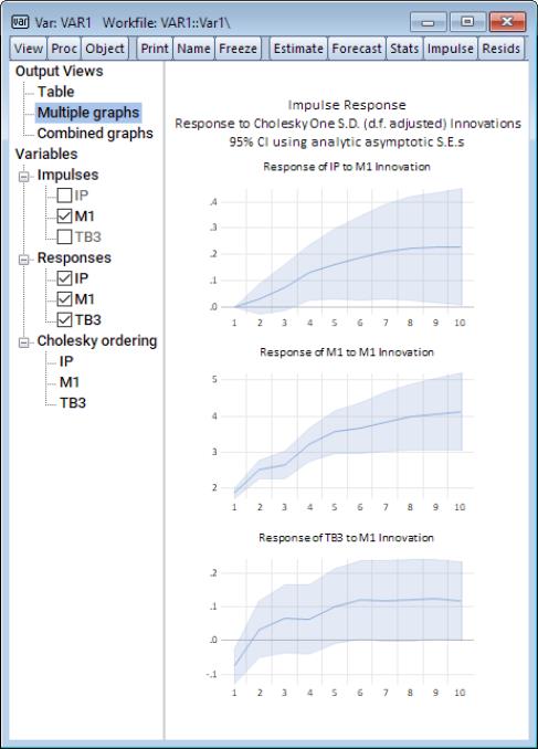
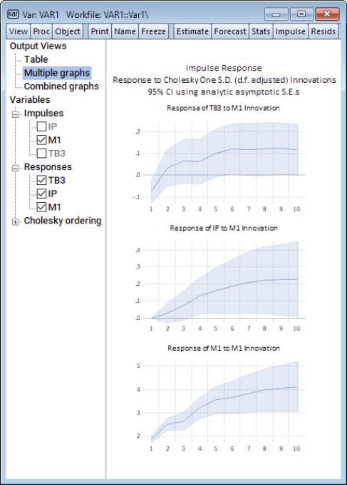
If we click the entries in the Impulses node for IP and TB3 to remove the checkmark next to them and click on Multiple graphs, the view will change to show only responses to the M1 impulses:
We may click-and-drag the TB3 entry in the Responses node to rearrange the order of the graphs