Data Handling
Statistics Canada (StatCan SDMX) Database Connectivity
EViews 14 offers easy-to-use connectivity to online databases from Statistics Canada, the Canadian national statistical office through EViews’ enhanced SDMX interface (
“Statistical Data and Metadata eXchange (SDMX) Databases”).
StatCan SDMX is not available in EViews Standard Edition.
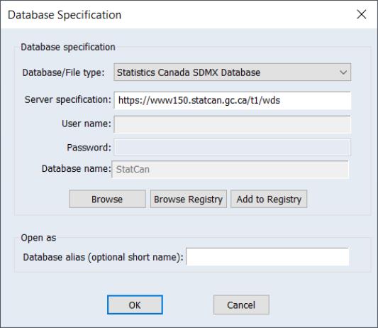
To begin, open the database windows by selecting File/Open Database from the primary EViews menu, select from the Database/File type drop down menu,
Click on to proceed and open the data browser
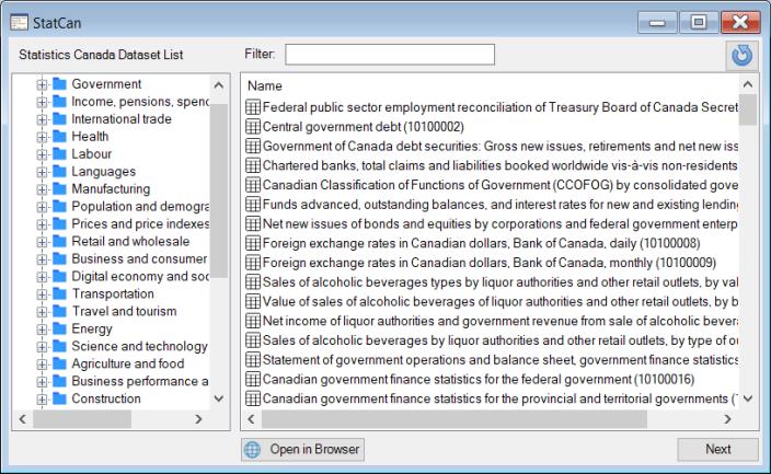
The left-hand side of the data browser offers tree interface through which may navigate until you locate the desired dataset.
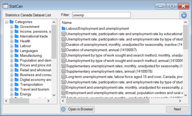
Alternately, you may use the Filter edit box to input a keyword, enabling a search across all categories and datasets.
Once you locate the desired dataset, you can either double-click on the dataset in the list on the right section or select it and then click Next to display the filter page.
Note that the StatCan SDMX databases offers a data browser on their official website that allows you to search for a dataset. Click on the Open in Browser button, which will open a web browser window showing the official database website.
To enhance the performance of the data explorer interface, categorization information is cached when the interface is first loaded. While a remote possibility, the database information may be updated during your EViews session. To refresh the cache, you may click on circular arrow Refresh button in the upper-right hand portion of the dialog.
You may use the filter page to refine your search. See
“Selecting Series” for additional detail. Once you have the data series desired, you may click on to download the data into an EViews workfile.
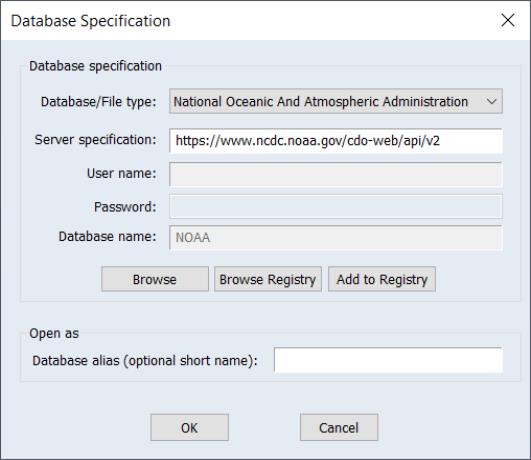
NOAA (National Oceanic And Atmospheric Administration)
The National Oceanic and Atmospheric Administration (NOAA) offers an extensive range of publicly available weather and climate datasets. For further details on NOAA data offerings, refer to:
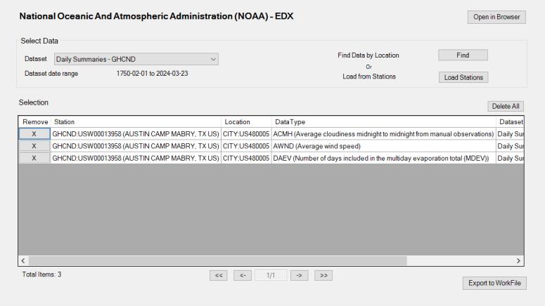
EViews 14 offers an all new interface that enables users to interact with EViews while simultaneously searching for data through the EDX dialog. This new NOAA database dialog includes a user-friendly table where all selected entries for import are recorded, facilitating the direct importation into a workfile. This process significantly enhances user workflow and efficiency, providing a seamless experience for data retrieval and integration into EViews.
To access the NOAA database, choose File/Open Database from the main EViews menu, and then select from the Database/File type drop down menu.
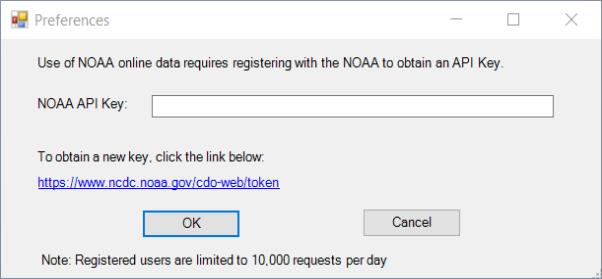
When opening the NOAA database for the first time, you'll be asked to enter an API Key obtained from the National Oceanic and Atmospheric Administration.
Enter your API key and click OK. The key will be saved as a user specific setting in your EViews “.ini” file. If you need to change the key later, select View/Preferences from the EViews database menu to modify your settings.
When you click on OK, EViews will open a standard database window.
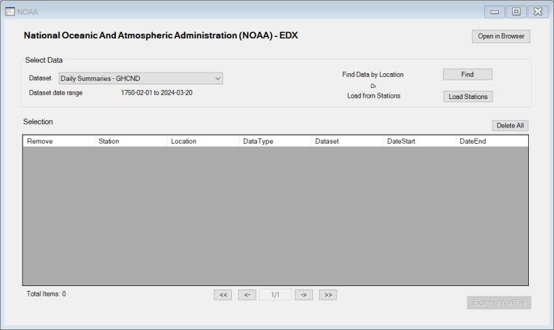
Click on Browse to open the custom NOAA window:
This custom interface will allow us to drill down through dataset, location, data type, and station selection to specify the data of interest.
When you first display this dialog, the area will be empty.
To select the data, first specify a dataset using the Dataset drop down menu.
You may then choose to Fi by clicking on the button to select one or more locations from a list, or you elect to Load from Stations by clicking on the button to specify stations using Station IDs.
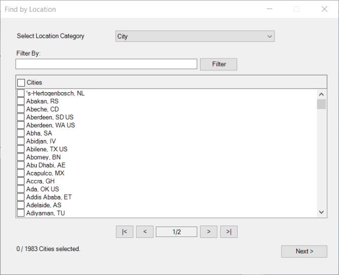
Find Data By Location
If you choose click on the button to Fi, a dialog will be displayed to walk you through the selection process:
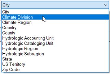
The drop down menu at the top should be used to specify a Location Category to browse:
You may choose from a variety of location categories including, for example, , , , , and .
You can filter the displayed list of locations using a text string by entering the text in the edit field, and clicking on the button.
Select the desired locations from the list and click Next to continue.
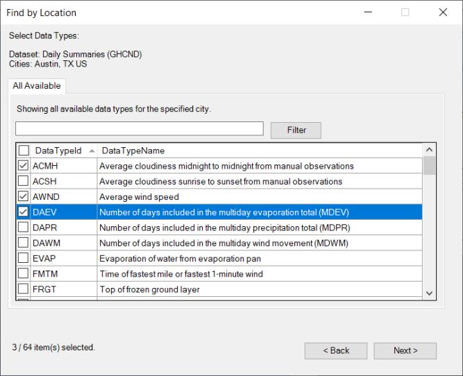
If you select a single location, you will see a dialog prompting you to select specific data types for the selected location:
You may use the filter to pare the list if desired. Click to select and deselect the entries.
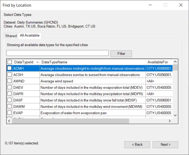
If you selected multiple locations in the location step, a EViews will display a dialog with two tabs: a Shared tab showing data types common to all of the locations, and an All Available tab listing all available data types across all of the locations.
Use the Filter edit field and button to refine your search in the lists on both tabs, select the data types of interest, and click Next to view the available NOAA stations.
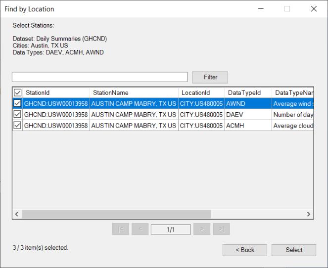
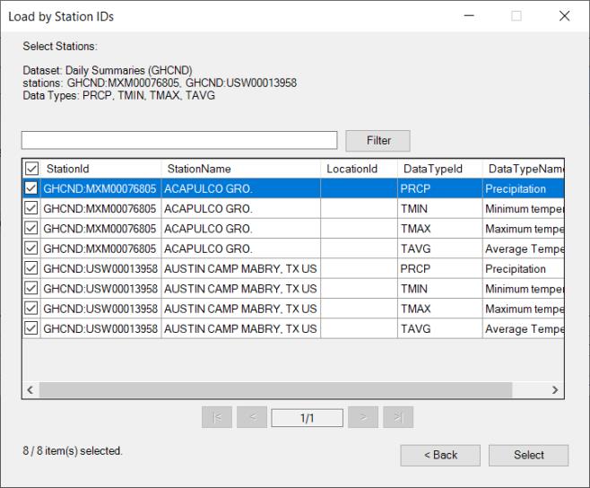
In the next dialog, you will find the available stations that match the selected data types and locations.
Choose the desired stations from which you want get data and the click Select.
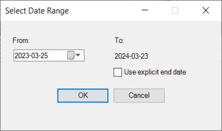
You will be asked to select a date range in order to limit the data results. NOAA restricts requests for annual and monthly data to a ten-year range; all other frequencies are restricted to a one-year range.
Click on to continue and display the main NOAA dialog:
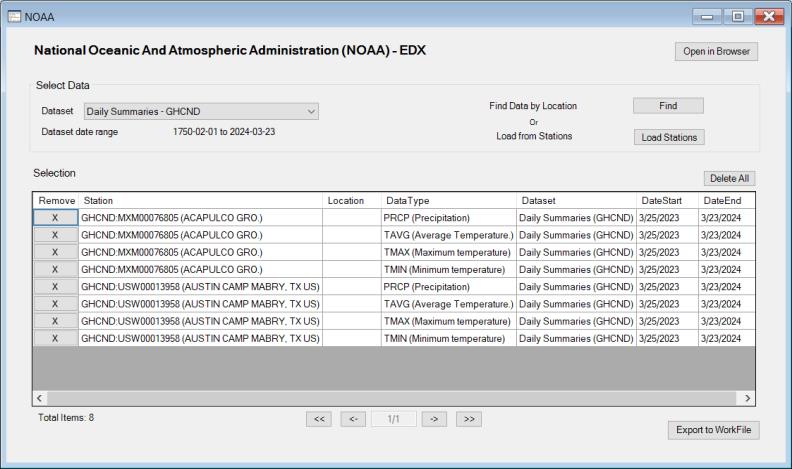
You will see in the Selection table the data you have just selected from your search. You can directly export these data to a workfile or find additional data before proceeding with the export.
Locations From Stations
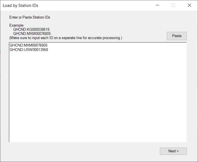
If you select Load Stations, instead of Find by Location, the displayed dialog will contain a textbox where you can manually type or paste from the clipboard the station IDs from which you want to retrieve data:
Click on to continue.
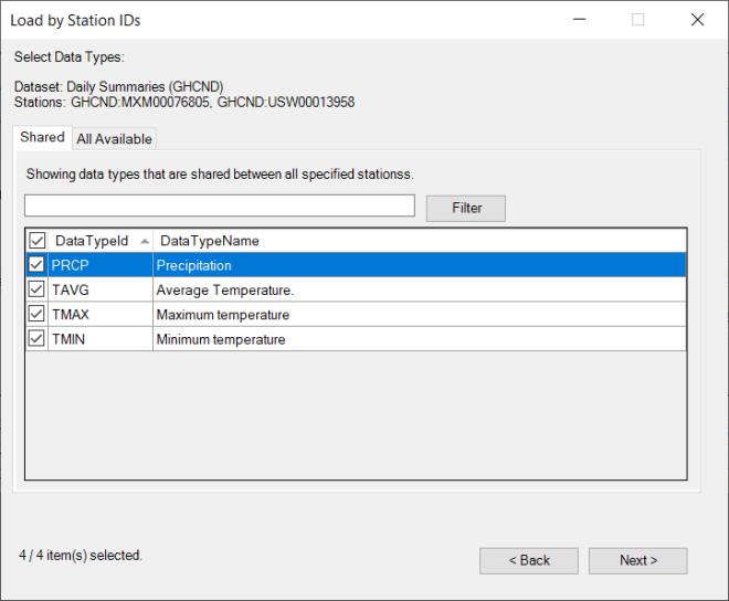
The next dialog will prompt you to select the data types. Once again, the dialog will feature one tab if there is a single location, or two tabs, a Shared tab for data types common to all of the locations, and an All Available tab for available data types across all of the locations.
Select the desired data types and click Next to display the next dialog where you will to select station and data type combinations:
Click on Select to continue to the final dialog where you will choose the date range:
As before, note that NOAA restricts requests for annual and monthly data to a ten-year range; all other frequencies are restricted to a one-year range.
Click on to continue and display the main NOAA dialog:
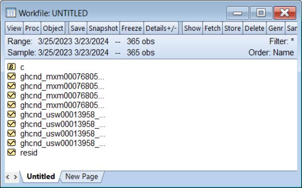
Click the Export to WorkFile button to export the chosen data to either an existing or a new workfile.
Statistical Data and Metadata eXchange (SDMX) Databases
EViews 14 offers a new, graphical user interface (GUI) designed for navigation and retrieval of data from SDMX databases.
The GUI browser for SDMX has undergone improvements to enhance user interaction. The introduction of category-based search functionality allows users to select datasets by their topics of interest, enabling more efficient searches across categories.
Additionally, several enhancements have been made to the series visualization window, including an improved filter search that enables users to select filters before initiating a search, significantly enhancing the speed of the process compared to previous versions. Moreover, efficiency improvements in data loading have been implemented, resulting in more responsive data loading.
SDMX Databases contain a large range of publicly available data. EViews offers direct access to the following online SDMX databases:
Please note that an internet connection is required to obtain SDMX online data. For more information on the datasets, please see the links above.
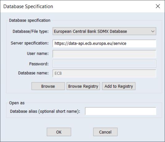
To begin, open the database windows by selecting File/Open Database from the primary EViews menu, select the desired SDMX database from the Database/File type drop down menu,
and click on OK to continue.
EViews displays the standard database dialog, indicating that you have an active connection to the data.
Click on Browse or Browse-Append to open the database.
Selecting a Database
EViews offers one of two different interfaces for selecting a SDMX database: a tree structure navigator and filter for databases that offer dataset categorization information, and a simple scroll and filter interface for databases without categorization information.
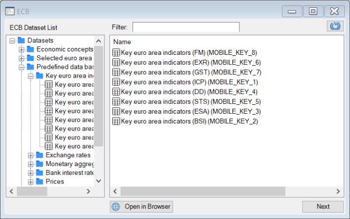
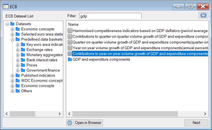
Categorized Datasets
If the SDMX database offers categorized datasets, the dialog interface offers features that facilitate dataset exploration through a nested tree structure.
The tree interface makes it easy to select or search for a specific category and then navigate through the nested tree until you locate the desired dataset. Simply use the tree structure on the left-hand pane to drill down to the desired subcategory, clicking on the node indicators as needed to inspect the contents. You may also double click on folders displayed in the right-hand pane to show its contents.
Alternatively, you can use the Filter edit box to input a keyword, enabling a search across all categories and datasets.
Once you locate the desired dataset, you can either double-click on the dataset in the list on the right section or select it and then click Next.
Some SDMX databases offer a data browser on their official website that allows you to perform more advanced search. Click on the Open in Browser button, which will open a web browser window showing the official database website.
To enhance the performance of the data explorer interface, categorization information is cached when the SDMX interface is first loaded. While a remote possibility, the database information may be updated during your EViews session. To refresh the cache, you may click on circular arrow Refresh button in the upper-right hand portion of the dialog.
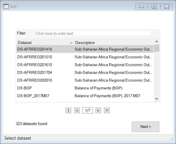
Non-Categorized Datasets
Alternatively, for SDMX databases that do not offer categorization information, the dialog interface simply offers a list of the available databases:
You can type a keyword in the Filter edit field to find a dataset. Select the dataset and click Next to continue.
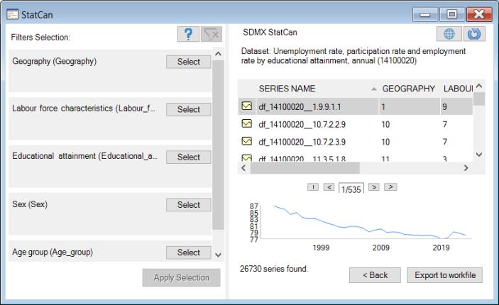
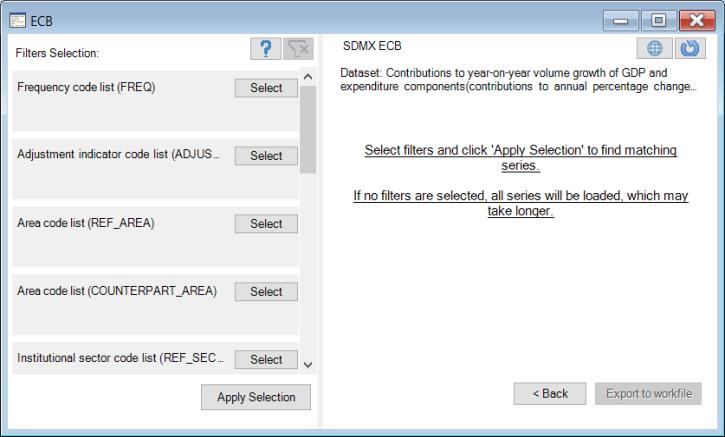
Selecting Series
In this dialog, you will choose the series to import:
We begin by forming a list of potentially relevant series. By default, all of the series in the dataset will be in the list. If available, you may use filters on the left-hand side of the dialog to reduce the number of series to be read. To specify a filter, click on the button on the left-hand side of the dialog corresponding to a specific category. You will be presented with a dialog showing the possible filter elements:
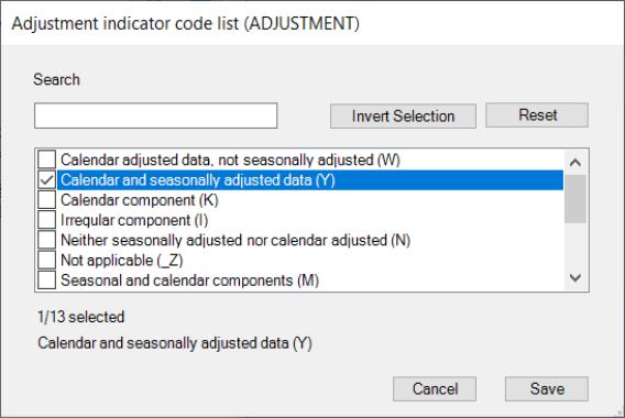
Click on the filter element entry to toggle the selection. You may use the button to locate a specific filter entry.
Here we use the to require data to be calendar and seasonally adjusted data:
Once the filter definition for the category is complete, click Save to save the filter settings and return the main selection dialog.
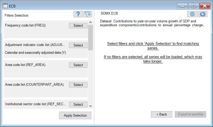
The dialog lists any relevant filter elements in text form under the name of the filter. If the information is not fully legible, you may hover your cursor over the text to see the full specification.
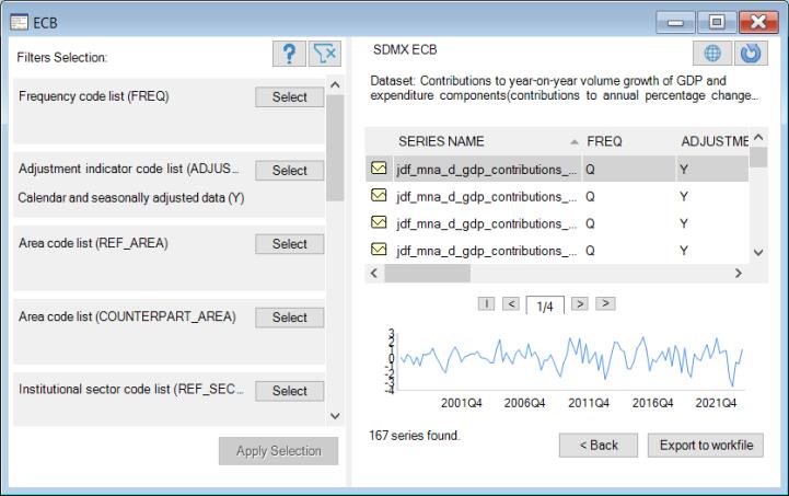
Once you finish defining any selection filters, click on the button to load a list of the relevant series in the dataset:
Here, there are 167 series found in the dataset that match the current filter. Click on any of the entries on the right to display information about the individual series and to display a thumbnail graph of the series.
You may go back and specify additional filters and click on the button to update the list of relevant series.
Finally, you may select one or more series in the list, then click on the Export to workfile button to load the selected series into a new or existing workfile.
Note that the Refresh Data button in the upper-right corner may be used to ensure the database information is up-to-date. For some databases, there will also be an Open in Browser button which will take you to the selected dataset on the database website if available. This feature is applicable only to those databases that offer an online data browser.
JDemetra+ Seasonal Adjustment
JDemetra+ is an open-source seasonal adjustment and time-series analysis package created by the European Commission. EViews incorporates a subset of the functionality provided by JDemetra+ to perform X-13 style seasonal adjustment on monthly and quarterly data.
While the results provided JDemetra+ will often be numerically identical to the results provided by Census X-13 (for identical settings), JDemetra+ offers robust handling of missing or extreme values, and computes the seasonal adjustment with reduced processing time.
When accessed from within EViews, JDemetra+ will perform seasonal adjustment on the series over the current workfile sample. In contrast to other seasonal adjustment methods, JDemetra+ offers automatic handling of missing values:
• For internal missing values (those not at the start or end of the sample), JDemetra+ uses interpolation to fill in the missing values.
• For missing values at the beginning or end of the sample, EViews will adjust the start and end of the adjustment sample. While JDemetra+ permits extrapolation of missing values at the beginning and end of the sample, EViews simply the trims the sample to remove NAs before sending the data to JDemetra+.
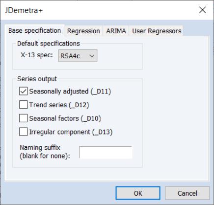
To perform JDemetra+ seasonal adjustment in EViews, click on Proc/Seasonal Adjustment/JDemetra+... from the series window menu in a monthly or quarterly workfile. This will open the JDemetra+ tabbed dialog:
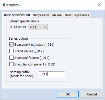
The first tab, Base specification allows you to choose one of the JDemetra+ preset specifications, as well as selecting which series to output into the workfile, and optionally specifying a suffix to be used in naming the output series.
• The X-13 spec: drop down menu specifies the preset specification. JDemetra+ offers a number of specifications with settings for the pre-treatment and decomposition steps of the seasonal adjustment:
| | | | |
X-11 | None | None | None | None |
RSA0 | None | None | None | Airline (0,1,1)(0,1,1) |
RSA1 | Automatic | AO/LS/TC | None | Airline (0,1,1)(0,1,1) |
RSA2c | Automatic | AO/LS/TC | TD2 (weekdays vs week-ends), Easter | Airline (0,1,1)(0,1,1) |
RSA3 | Automatic | AO/LS/TC | None | Automatic selection |
RSA4c | Automatic | AO/LS/TC | TD2 (weekdays vs week-ends), Easter | Automatic selection |
RSA5 | Automatic | AO/LS/TC | TD7 (7 day of week variables), Easter | Automatic selection |
For in-depth details of these specifications, we recommend browsing the JDemetra+
website (https://github.com/jdemetra).
• The Mode: dropdown specifies the X-11 decomposition mode that will be used. JDemetra+ only allows the user to specify the decomposition mode if no pre-adjustment is being performed, so this dropdown is only enabled when the X-11 default specification is selected.
• The Series output section specifies which of the output series from JDemetra+ will be exported to the workfile. By default, each output series will be created a name equal to that of the underlying series plus the type of series being created (e.g., if JDemetra+ is run on the series GDP, then the seasonally adjusted D11 series will be created with a name of GDP_D11). You can use the Naming suffix edit field to enter an additional suffix that will be appended to the series name before the output type (e.g., if you enter “_JD” as the Naming suffix then the D11 series for GDP will be created with a name of GDP_JD_D11).
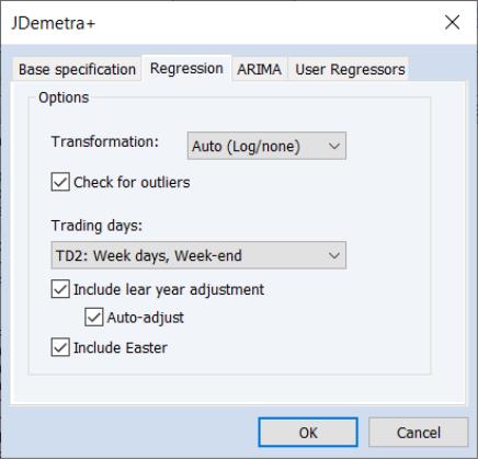
The Regression tab of the dialog allows you to override some of the options set by the default specifications relating to the pre-adjustment regression step of X-13 style seasonal adjustment.
Selecting the X-13 specification on the Base specification tab will change the settings on this tab, but you can fine tune the default settings by using the options on this tab.
• The Transformation drop down menu specifies whether a log transformation should be applied to the underlying series before running the regression. Auto (Log/none) instructs JDemetra+ to automatically detect whether a log transform should be applied or not.
• The Check for outliers check box specifies whether JDemetra+ should automatically detect outliers. EViews' implementation of JDemetra+ supports only the Additive Outlier (AO), Level Shift (LS), and Temporary Change (TC) types of outliers, and when the option is checked, JDemetra+ will detect for all three types simultaneously.
• Trading days sets the type of calendar effects used in the pre-adjustment regression. These effects consist of created variables with the count of the number of days in each period. The options are:
| |
TD7 | Create 7 calendar variables. The first counts the number of Mondays in the month/quarter. The second counts the number of Tuesdays, and so on. |
TD4 | Create 4 calendar variables. The first counts the number of days from Monday to Thursday, the second counts the number of Fridays, the third counts Saturdays, and the fourth counts Sundays. |
TD3c | Create 3 calendar variables. The first counts the number of days from Monday to Thursday, the second counts the number of Fridays and Saturdays, and the third counts Sundays. |
TD3 | Create 3 calendar variables. The first counts the number of days from Monday to Friday, the second counts the number of Saturdays, and the third counts Sundays. |
TD2 | Create 2 calendar variables. The first counts the number of week days (Mon-Fri) and the second counts the number of weekend days (Sat-Sun). |
TD2c | Create 2 calendar variables. The first counts the number of days from Monday to Saturday, and the second counts the number of Sundays. |
User variables | Include user-provided calendar variables only. |
The created variables are compacted into a single calendar variable through a transformation. For example, TD2 creates the calendar variable as NumWeekDays-(5/2)*NumWeekends.
If User variables is selected as the trading day type, you must specify series to use as calendar variables on the User Regressors tab.
• The Include Leap Year adjustment and Include Easter checkboxes control whether additional adjustments are made to the calendar effects for the impact of leap years and Easter. The Auto-adjust checkbox specifies whether JDemetra will automatically determine whether to drop the leap-year adjustment.
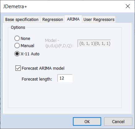
The ARIMA tab provides options for the estimation of the ARIMA model in the pre-adjustment step:
• The ARIMA Method section selects the method used to specify the ARIMA model to be estimated. None instructs JDemetra+ to not estimate an ARIMA model at all.
If Manual is selected, you can enter a specific ARIMA order in (p, d, q)(P, D, Q) notation, where p is the AR order, d is the differencing level, q is the MA order, P is the seasonal AR order, D is the seasonal differencing level, and Q is the seasonal MA order.
If X-11 Auto is selected, JDemetra+ will use its default X-11 selection routine to select the most appropriate ARIMA order.
• The Forecast ARIMA model checkbox instructs JDemetra+ to forecast the ARIMA model beyond the end of the series. The number of periods forecasted can be changed using the Forecast length edit field. Forecasting the ARIMA model allows JDemetra+ to provide forecasts of the final seasonally adjusted series and seasonal factors. Note forecasts will only be imported into EViews if the workfile range covers the period of the forecast.
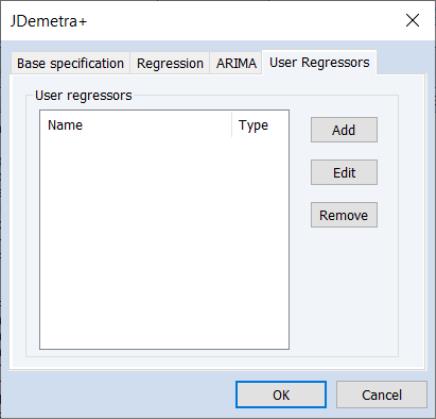
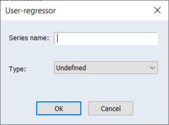
The User Regressors tab of the dialog supports providing user-provided exogenous series to the pre-adjustment ARIMA/regression models.
Clicking on the Add button brings up a dialog asking you to type in the name of the workfile variable that you would like to include as a regressor:
You may enter any valid EViews series name or expression, such as "X" or "log(X)", or "@pch(X)" in the edit field. You may also type in a space delimited list to add multiple series at once.
The drop down menu should be used to specify a regressor type for the variable you are including (i.e., , , , etc.). Changing the type of the regressors changes the exact impact that series has on the final seasonal adjustment calculation. The JDemetra+ documentation has details on the exact calculations.
If you selected User Variables as the Trading Days type, you must add at least one user-regressor with a type of Calendar/TradingDay.
Example
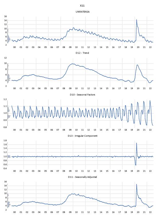
The workfile, "X13_Macro.wf1" includes a series called UNRATENSA which contains monthly non-seasonally adjusted US unemployment data from January 2005 to June 2012. We will use this series to demonstrate the user of JDemetra+ seasonal adjustment in EViews. We will later use the same series to demonstrate X-13 seasonal adjustment.
We will perform simple X-11 based seasonal adjustment on this series without any pre-adjustment regression options being set. To do so open the UNRATENSA series and click on to open the JDemetra+ dialog.
Simple X-11 adjustment is one of the pre-set JDemetra+ defaults, so we change the X-13 spec: dropdown to X-11. We'll elect to store the seasonally adjusted values in the workfile, and enter “_x11” in the edit field:
Clicking to display the JDemetra+ graph output:
The output is split into five graphs. The top graph displays the original unadjusted series. The second displays the decomposed trend line, the third the seasonal/cyclical factors, the fourth the irregular/residual component, and finally graph displays the seasonally adjusted values. It should be noted that this simple X-11 adjustment via JDemetra+ will give numerically identical results to using EViews’ implementation of Census X-13 using the default settings.
Boosted Hodrick-Prescott Filter
The Hodrick-Prescott Filter is a widely employed smoothing method for obtaining a smooth estimate of the long-term trend component of a series. The method was first proposed in a working paper (circulated in the early 1980’s and published in 1997) by Hodrick and Prescott to analyze postwar U.S. business cycles.
EViews 14 enhances the existing routines with support for the iterated (boosted) HP filter proposed by Phillips and Shi (2020).
Technically, the Hodrick-Prescott (HP) filter is a two-sided linear filter that computes the smoothed series

of

by minimizing the variance of

around

, subject to a penalty that constrains the second difference of

. The HP filter chooses the values of

to minimize:
 | (0.1) |
The

series is often referred to as the trend series. The cyclical component

of the original series can be computed as

.
The penalty parameter

controls the smoothness of

. The larger the

, the smoother the

. As

,

approaches a linear trend.
Phillips and Shi (2020) have proposed iterating the HP filter to produce a “smarter smoothing device.” This
boosted HP filter takes the cyclical series,

and runs the filter on it one more time to produce a new smoothed and cycle series. The filtering process is repeated, producing a further smoothed series at each iteration. The advantage of this iterative procedure is that the final smoothed series is less reliant on the choice of

. Phillips and Shi recommend repeating the process either after a set number of iterations, or through the use of information criteria to decide the optimal number of iterations.
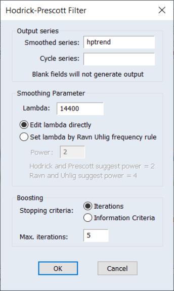
To smooth the series using the Hodrick-Prescott filter, choose :
First, provide a name for the . EViews will suggest a name, but you can always enter a name of your choosing. If you wish to save a , specify a name in the edit field.
Next, specify an integer value for the smoothing parameter,

. You may specify

directly by clicking on the radio button and entering a value in the edit field, or you may specify a value using the frequency power rule of Ravn and Uhlig (2002) (the number of periods per year divided by 4, raised to a power, and multiplied by 1600 by clicking on the and entering a value in the edit field.
By default, EViews will fill the defaults using the Ravn and Uhlig method with a power rule of 2, yielding the original Hodrick and Prescott values for

:
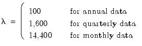 | (0.2) |
Ravn and Uhlig recommend using a power value of 4. EViews will round any non-integer values that you enter.
The Boosting section of the dialog offers settings for iterative boosting of the HP filter. You may choose between stopping based on the maximum number of iterations or using an Information criteria.
If you click on , EViews will stop based on the entry in the Max. Iterations edit field. By default, there will be no boosting as only one iteration of the filter will be performed.
Selecting the Information criteria radio button instructs EViews to select the optimal number of iterations using information criteria. The Max. Iterations edit field should be used to specify the number of iterations to be considered.
When you click on OK, EViews displays a graph of the filtered series together with the original series. Note that only data in the current workfile sample are filtered. Observations for the smoothed and cyclical series outside the current sample will be filled with NAs.
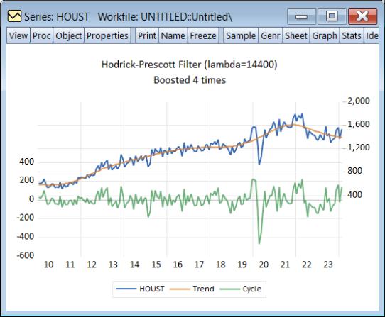
For example, we may download housing starts data from the Federal Reserve of St. Louis database:
dbopen(type=fred, server=api.stlouisfed.org/fred)
wfcreate m 1959M01 2024M02
fetch(d=fred) houst
smpl 2010 2024m02
and then perform HP filtering with 5 iterations on the HOUST series using values from 2010m01 through 2024m02:
The newly created HPTREND series contains the smoothed values of HOUST.