Function Reference: Q
@qbeta Beta distribution quantile.
@qbinom Binomial distribution quantile.
@qchisq Chi-square distribution quantile.
@qexp Exponential distribution quantile.
@qextreme Extreme value (Type I-minimum) distribution quantile.
@qgamma Gamma distribution quantile.
@qged Generalized error distribution quantile.
@qnegbin Negative binomial distribution quantile.
@qnorm Standard normal distribution quantile.
@qtdist Student’s

distribution quantile.
@quantilesby Empirical quantiles of a series for each specified group.
@quarter Quarter of the year of the observation.
@qunif Uniform distribution quantile.
@qweib Weibull distribution quantile.
Beta distribution quantile.
Syntax: @qbeta(p, a, b)
p: number,

a: number,

b: number,

Return: number
Find the x satisfying
where
and 0 elsewhere, and

is the beta function
Examples
= @qbeta(0.75, 1, 2)
returns 0.5.
Cross-references
See also
@cbeta,
@dbeta, and
@rbeta.
Binomial distribution quantile.
Syntax: @qbinom(v, n, p)
v: number,

n: integer,

p: number,

Return: integer
Find value with cumulative probability exceeding

.
Returns smallest integer

satisfying
 where
whereis the cumulative probability function evaluated at
 ,
, Examples
= @qbinom(0.5, 5, 0.5)
returns 2.
Cross-references
Chi-square distribution quantile.
Syntax: @qchisq(p, v)
p: number,

v: number,

Return: number
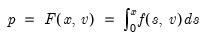
Find the x satisfying
where
Examples
= @qchisq(0.5, 100)
returns 99.33412....
Cross-references
Exponential distribution quantile.
Syntax: @qexp(p, m)
p: number,

m: number,

Return: number
Return the

satisfying
so that
Examples
= @qexp(0.5, 1)
returns 0.69314... (equal to log(2)).
Cross-references
See also
@cexp,
@dexp, and
@rexp.
Extreme value (Type I-minimum) distribution quantile.
Syntax: @qextreme(p)
p: number,

Return: number
Return the

satisfying
so that
Examples
= @qextreme(0.5)
returns -0.36651....
Cross-references
F-distribution quantile.
Syntax:
@qfdist(
p,  ,
,  )
) p: number

: number,


: number,

Return: number
For

, find the
x satisfying
where,
for

and 0 otherwise, and

is the beta function
Examples
= @qfdist(0.5, 2, 2)
returns 1.
Cross-references
Quadratic form.
Syntax: @qform(s, o)
s: sym
o: vector, matrix, sym
Return: number, sym
Returns the quadratic form of a symmetric matrix s, with a vector or matrix object o.
• if o is a vector, the function returns a scalar
• If o is a matrix, the function returns a sym
Examples
sym s1 = @inner(@mnrnd(20, 4))
vector v1 = @mrnd(4)
scalar q1 = @qform(@inverse(s1), v1)
generates a symmetric matrix S1, then computes the quadratic form using the inverse of S1, and the randomly generated vector V1.
matrix m1 = @mrnd(4, 5)
sym q2 = @qform(@inverse(s1), m1)
computes the matrix form of the quadratic form, returning a sym.
Cross-references
See also
@inner and
@outer.
Gamma distribution quantile.
Syntax: @qgamma(p, b, r)
p: number,

b: number,

r: number,

Return: number
Return the

satisfying
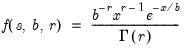
where
for

and 0 elsewhere.
Examples
= @qgamma(0.5, 4, 1)
returns 2.77258....
Cross-references
Generalized error distribution quantile.
Syntax: @qchisq(p, r)
p: number,

r: number,

Return: number
Find the x satisfying
where
Examples
= @qged(0.75, 2)
returns 0.67448....
Cross-references
See also
@cged,
@dged, and
@rged.
Laplace distribution quantile.
Syntax: @qlaplace(p)
p: number
Return: number
Return the

satisfying
where
Examples
= @qlaplace(0.25)
returns -0.69314....
Cross-references
Logistic distribution quantile.
Syntax: @qlogistic(p)
p: number,

Return: number
Return the

satisfying
so that
Examples
= @qlogistic(0.5)
returns 0.
Cross-references
Log normal distribution quantile.
Syntax: @qchisq(p, m, s)
p: number,

m: number,

s: number,

Return: number
Find the x satisfying
where
Examples
= @qlognorm(0.5, 0, 2)
returns 1.
Cross-references
Negative binomial distribution quantile.
Syntax: @qnegbin(v, n, p)
v: number,

n: number,

p: number,

Return: integer
Find value with cumulative probability exceeding

.
Returns smallest integer

satisfying
 where
whereis the cumulative probability function evaluated at
 ,
, Examples
= @qnegbin(0.5, 10, 0.5)
returns 9.
Cross-references
Standard normal distribution quantile.
Syntax: @qnorm(p)
p: number
Return: number
Return the

satisfying
where
Examples
= @qnorm(0.95)
returns 1.64485....
Cross-references
Pareto distribution quantile.
Syntax: @qpareto(p, m, a)
p: number,

m: number,

a: number,

Return: number
Return the

satisfying
Examples
= @qpareto(0.75, 1, 2)
returns 2.
Cross-references
Poisson distribution quantiles.
Syntax: @qpoisson(p, m)
p: number,

m: number,

Return: integer
Find value with cumulative probability exceeding

.
Returns smallest integer

satisfying
 where
whereis the cumulative probability function evaluated at
 ,
, Examples
= @qpoisson(0.5, 10)
returns 10.
Cross-references
QR decomposition.
Syntax: @qr(M, R[, P])
M: matrix
R: matrix
P: (optional) matrix
Return: matrix

Decomposes an

matrix

into an

orthogonal matrix

and an

upper triangular matrix

such that

, where

.
If permutation matrix

is provided, the decomposition produces

and

such that

.
Examples
matrix m1 = @mnrnd(7, 5)
matrix r
matrix q = @qr(m1, r)
generates a random matrix M1, then decomposes it into the orthogonal matrix Q, and the upper triangular matrix R.
The following illustrate the properties of the decomposition:
sym i1 = @inner(q)
matrix m2 = q * r
where I1 is the identity matrix, and M2 is equal to M1.
Cross-references
Student’s

distribution quantile.
Syntax: @qtdist(p, v)
p: number,

v: number,

Return: number
Return the

satisfying
where
Examples
= @qtdist(0.025, 1)
returns -12.70620....
Cross-references
Empirical quantile.
Compute the quantile value where approximately 100*q percent of the data is less than or equal to the value,
Syntax: @quantile(x, q[, m, s])
x: series, vector, matrix
q: number, series, vector, matrix
m: (optional) string
s: (optional) sample string or object when x is a series and assigning to a series
Return: number
• The quantile value
q must satisfy

.
• m is an optional string controlling the method of calculating the empirical distribution function: “b” (Blom), “r” (Rankit-Cleveland), “o” (Ordinary), “t” (Tukey), “v” (van der Waerden), “g” (Gumbel). The default value is “r”.
Rankit-Cleveland (default) | |
Ordinary | |
Van der Waerden | |
Blom | |
Tukey | |
Gumbel | |
To compute the

-quantile, first find

, the smallest rank such that,
where the order statistics

represent data for the

observations ordered from low to high, and

is the assumed empirical distribution function. For purposes of computing

, tied ranks are assumed to take the last tied value.
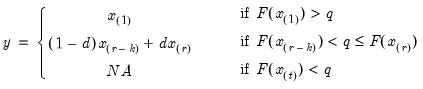
Then the quantile is computed as
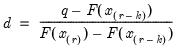
where the interpolating constant is
for

the smallest integer where

. In the leading case where there are no tied

values,

.
For series calculations, EViews will use the current or specified workfile sample.
Examples
= @quantile(x, 0.5)
returns the median of the series x.
= @quantile(x, 0.1)
returns the first decile (10th percentile) of the series x.
Cross-references
Empirical quantiles of a series for each specified group.
Syntax: @quantilesby(x, y[y1, y2, ... yn], q, [s])
x: series
y: series, alpha
q number
s: (optional) sample string or object
Return: series
Returns the
q-th quantile of
x for each group defined by distinct values of y. The quantiles will be computed using the Rankit-Cleveland definition (see
@quantile)
. EViews will use the current or specified workfile sample.
Examples
show @quantilesby(x, g1, g2, 0.25)
produces a linked series of the by-group 25th percentiles of the series x, where members of the same group have identical values for both g1 and g2.
Cross-references
Quarter of the year of the observation.
Syntax: @quarter
Return: series
Returns the quarter of the year (1–4) associated with each observation in the workfile.
• If the workfile is of lower than quarterly frequency, all observations will be set to 1.
• If the workfile is undated, observations will be set to -1.
Examples
series dt = @quarter
saves the quarter into the series DT.
The command
smpl if @quarter = 4
sets the sample to only include fourth quarter observations.
Cross-references
Uniform distribution quantile.
Syntax: @qunif(p, a, b)
p: number,

a: number
b: number,

Return: number
Return the

satisfying
so that
Examples
= @qunif(0.4, 1, 6)
returns 3.
Cross-references
See also
@cunif,
@dunif, and
@runif.
Weibull distribution quantile.
Syntax: @qweib(p, m, a)
p: number,

m: number,

a: number,

Return: number
Return the

satisfying
Examples
= @qweib(0.5, 1, 1)
returns 0.69314... (the natural log of 2).
Cross-references
See also
@cweib,
@dweib, and
@rweib.