Econometrics and Statistics
MIDAS GARCH
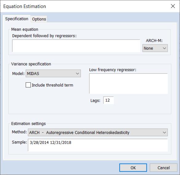
EViews 14 estimates the multiplicative component MIDAS GARCH(1,1) model of Conrad and Kleen (2020).
Mixed Data Sampling (MIDAS) regression is an estimation technique which allows for data sampled at different frequencies to be used in the same regression. For MIDAS GARCH models, the approach is to incorporate information from a large number of lags of a lower frequency series into the variance specification of an ARCH regression; incorporating, for example, lags of quarterly data in a monthly data GARCH model.
While most of the dialog should be familiar, the MIDAS GARCH variance specification uses lags of a low frequency regressor. You should enter the name of a single permanent component regressor in the Low frequency regressor edit field.
The syntax for specifying this variable is pagename\seriesname where pagename is the name of the page containing the series, and seriesname is the name of the series.
Note that EViews only allows the specification of a single low frequency regressor.
You should use the Lag edit field to specify the number of low frequency regressor lags to include in the permanent component.
Quantile ARDL Estimation
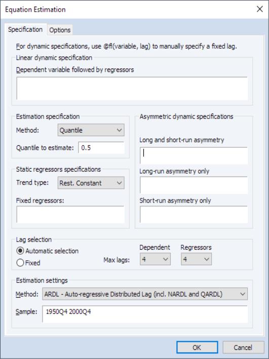
The Quantile Autoregressive Distributed Lag (QARDL) model, introduced by Cho, Kim, and Shin (2015), is an extension of traditional ARDL models to capture the dynamics of conditional quantiles (percentiles) of the dependent variable. While conventional models provide insights into the mean responses of the dependent variable to changes in predictors, QARDL models allow you to model the effects of changes in predictors on the quantiles of the dependent variable.
While QARDL models may be estimated using generic quantile regression tools by specifying models using with the appropriate levels, lags and lag differences of variables, EViews 14 offers an easy-to-use native interface for estimating QARDL and QNARDL models.
To estimate a QARDL or QNARDL model, select ARDL - Autoregressive Distributed Lag Models in the estimation Method drop down at the bottom of the dialog, and then select in the Estimation specification section in the middle of the left column:
Preliminary documentation for estimating Quantile ARDL is available. For primary documentation:
• See
Equation::ardl for updated command documentation for Quantile ARDL estimation.
There are new commands associated with Quantile ARDL views:
•
Equation::qrcrprocess displays a spool object producing a quantile process of the cointegrating relation.
•
Equation::qrecprocess displays a spool object producing a quantile process for each of the conditional error correction and error correction coefficients.
Enhanced Elastic Net and Lasso
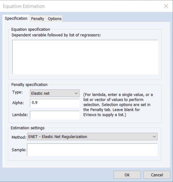
The elastic net (Enet) estimator performs penalized least squares regression with a penalty that depends on a parameterized function of the absolute and squared values of the coefficients. Notably, the class of Enet models includes the special cases of ridge and Lasso (Least Absolute Shrinkage and Selection Operator) regression.
While prior versions of EViews did offer tools for elastic net estimation, EViews 14 completely updates the existing features to offer more efficient algorithms for estimation, added control over coefficient penalties including individual coefficient weights and coefficient bounds, more efficient cross-validation tools for selecting models along the lambda path, and enhanced views and tools for examining the behavior of coefficients, estimation objectives, and model fit statistics along the path.
(Note that Enet equations estimated in EViews 14 are not backward compatible with earlier versions and these equations will not be read by previous versions. Conversely, Enet equations estimated in EViews 13 and prior will need to be re-estimated in EViews 14).
To estimate an elastic net model, select in the drop-down menu:
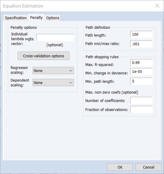
The page offers new settings for individual penalty weights, path definition, cross-validation, and variable scaling:
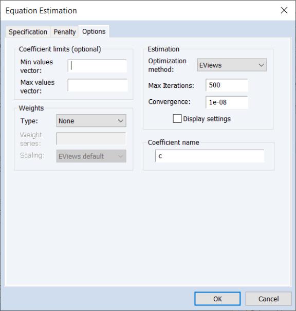
The page offers, among other things, new options for placing limits on coefficients, and optimization methods:
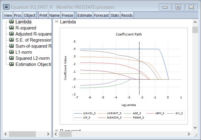
Once you have estimated a path model, EViews 14 offers improved views tools for examining the behavior of coefficients, estimation objectives, and model fit statistics along the path. Clicking on a spool object plotting coefficients against various values:
For additional discussion:
There are a number of new or improved commands associated with elastic net views:
•
Equation::coefpath – display graphs of the paths of the coefficients plotted against lambda, fit measures, and estimation values.
•
Equation::cvgraph – display a graph of the cross-validation objective against the lambda path.
•
Equation::lambdacoefs – display the spreadsheet of the matrix of coefficient values along the lambda path.
•
Equation::lambdaest – display the table showing various values associated with estimation along the lambda path.
•
Equation::lambdafit – display the table showing various fit statistics associated with estimates along the lambda path.
New equation data members have been introduced to provide access to the results of estimation and cross-validation:
Lasso Variable Selection
The Lasso variable selection (VARSEL) features in EViews have been updated to use the enhanced elastic net estimation features.
(Note that VARSEL equations estimated using Lasso in EViews 14 are not backward compatible with earlier versions and these equations will not be read by previous versions. Conversely, VARSEL equations estimated using Lasso from EViews 13 and prior will need to be re-estimated in EViews 14).
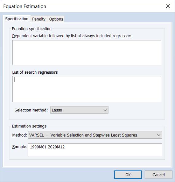
To perform a VARSEL using Lasso in EViews select or press from the toolbar of an existing equation. From the dialog choose and choose in the method drop down menu. EViews will display the following dialog:
Lasso Options
For Lasso selection, the there are two options dialog pages that allow you control the specification of the objective and the estimation method.
You may use the dialog pages to control the determination of the penalty parameter, to specify data transformation options, individual observation weights, and to control the iterative estimation procedure.
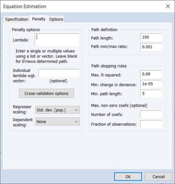
The first options page is the page:
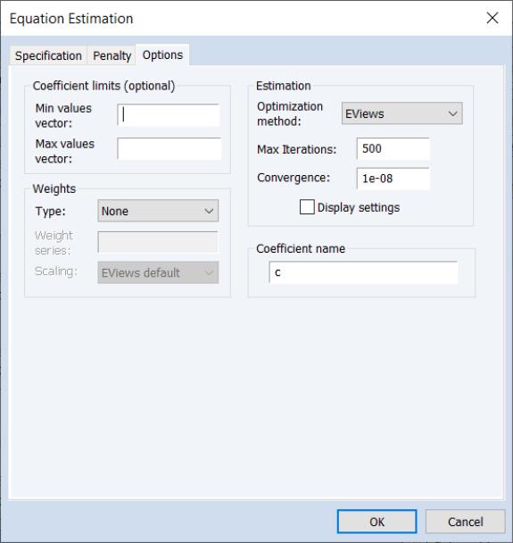
The second page allows you to set coefficient limits, add observation weights, control the estimation method and convergence, and to change the coefficient name:
The Varsel documentation has been updated to describe the new interface:
There are a number of new or improved commands associated with the Lasso variable seletion views:
•
Equation::coefpath – display graphs of the paths of the coefficients plotted against lambda, fit measures, and estimation values.
•
Equation::cvgraph – display a graph of the cross-validation objective against the lambda path.
•
Equation::lambdacoefs – display the spreadsheet of the matrix of coefficient values along the lambda path.
•
Equation::lambdaest – display the table showing various values associated with estimation along the lambda path.
•
Equation::lambdafit – display the table showing various fit statistics associated with estimates along the lambda path.
New equation data members have been introduced to provide access to the Lasso and model selection results:
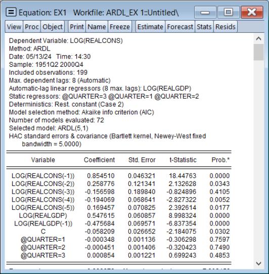
Expanded ARDL HAC Standard Errors
EViews 14 expands the calculation of heteroskedasticity and autocorrelation consistent (HAC) estimates of coefficient covariances in ARDL equations. Previously, HAC coefficient covariances were only computed for the base ARDL estimates of the Intertemporal Dynamics (ITD) representation of the specification. HAC estimates were not available for the Conditional Error Correction (CEC) or Error Correction (EC) forms of the model.
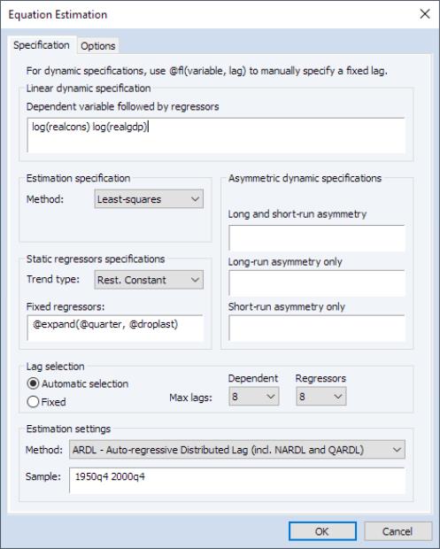
EViews now computes HAC estimates for all three representations.To estimate an ARDL model with HAC correction select or press from the toolbar of an existing equation.
From the dialog choose the in the dropdown to display the estimation dialog:
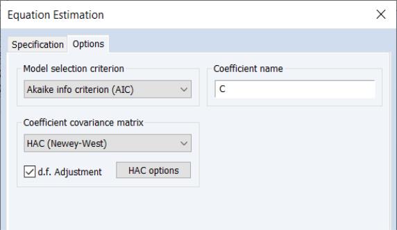
Fill on the page as desired, and then click on the tab to display the settings:
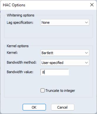
Select from the dropdown menu. You may click on the button to display a popup dialog that will allow you to change from the default settings:
If you change the , click on to accept the changes, then click on on the estimation dialog to estimate your ARDL with using the specification and options.
The IC results are displayed by default:
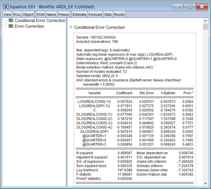
To see the CEC and the EC results, select to display the estimates for the alternative representations:
Note that the labeling of output in this view may have been misleading on prior versions of EViews as the comments related to estimation of coefficient covariances only applied to the ITD specification.
Facebook Prophet Forecasting
EViews 14 offers access to the powerful Facebook Prophet forecasting engine through a new, easy-to-use user interface.
By default, a custom Prophet Python package is installed in your EViews installation directory. If Prophet was not installed with EViews, you will need to reinstall EViews.
Background
The Prophet forecasting tool offers a flexible, easy-to-configure method of forecasting time series data. A particular emphasis of the Prophet design is its support for users with an understanding of the data-generating process but limited knowledge of time series methods, and its ability to produce a large number of forecasts with limited human intervention (Taylor and Letham 2018).
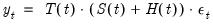
The original Prophet is a time series model which decomposes a series into additive trend, seasonal and holiday components:
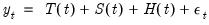 | (0.3) |
where

is the trend component,

represents periodic seasonal (weekly, monthly, yearly,
etc.) components,

represents potentially irregular holiday effects, and

is a normally distributed idiosyncratic error.
A multiplicative seasonal version of the Prophet model may be written as:
 | (0.4) |
The current EViews implementation supports the trend

and seasonal

components of the Prophet specification.
The specification of these components is described in some detail in Taylor and Letham (2018). Roughly speaking:
• The trend component

is modeled using a piecewise logistic or piecewise linear growth model with explicit change-points that may be specified or automatically determined. EViews supports automatic determination of change-points.
• The smooth seasonal component

is approximated using a linear combination of a set of Fourier series.
Estimation of the Prophet model employs Bayesian techniques with normal priors on the trend and seasonal Fourier series, and a Laplace prior on the change-points.
Using Prophet in EViews
To use Prophet in EViews to forecast a series, open the series and click on Proc/Automatic Forecasting/Prophet… which will bring up the Prophet Forecasting dialog.
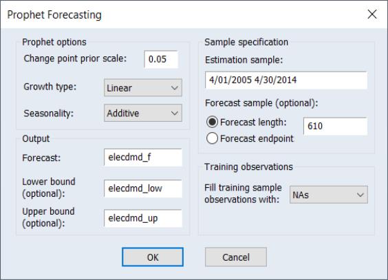
The Prophet options section of the dialog allows you to select some of the options offered by Prophet.
The Sample specification section of the dialog includes the Estimation Sample box and the Forecast length box.
• The Estimation Sample determines the observations used in training the Prophet model. By default, EViews will fill the dialog with the current workfile sample.
• Forecast length specifies h, the number of observations that will be forecast after training. The forecast sample will start immediately after the last observation of the estimation sample and will continue for h observations. Note the workfile must be sized such that h observations exist in the workfile after the estimation sample.
• As an alternative to Forecast length, you may specify a Forecast endpoint. The observation specified as the forecast endpoint must follow the last observation in the estimation sample and fall within the range of the workfile.
The Output section boxes are used to name the final forecast series in the workfile.
• You must provide a name for the output series. By default, edit field is filled with the name of the underlying series followed by an "_F".
• The optional Lower bound and Upper bound edit fields allow you to save the lower and upper forecast bounds computed by Prophet. By default, the edit fields are pre-filled with the name of the underlying series followed by “_LOW” and “UP”, respectively.
You may use the Training observations selection to specify how the forecast series' observations within the training sample will be filled in. By default, EViews overwrites the in-sample forecast values with NAs. You may instead instruct EViews to use the Prophet computed in-sample forecast for the training sample values, or to use the underlying series actual values. Any observations that are neither in the training sample nor the forecast sample will be filled with NAs.
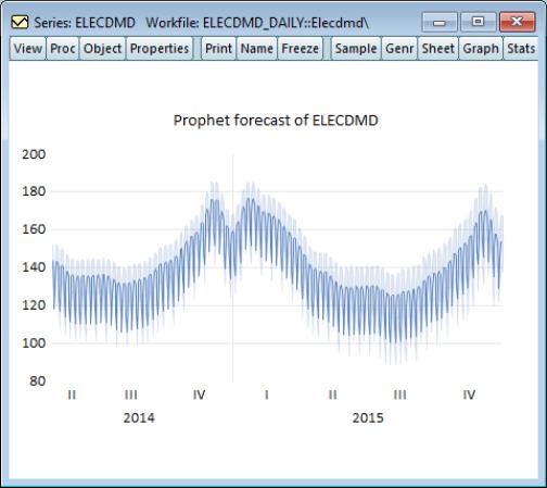
Example
As an example of using Prophet in EViews, we forecast daily electricity demand in England and Wales, using the workfile "elecdmd_daily.wf1". This workfile contains monthly electricity demand data from April 2005 until April 2014 (in the series ELECDMD). The workfile's range extends through the end of 2015, even though data for ELECDMD is only available until April 2014.
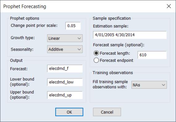
To use Prophet to forecast the missing values, we open the ELECDMD series and click on Proc/Automatic Forecasting/Prophet… to bring up the Prophet dialog:
EViews automatically fills in the estimation sample to the current workfile sample (which was set to the actual data of ELECDMD), and calculates the forecast length based on the number of remaining observations.
We leave all other options at their default value and click OK to produce the forecast:
The Facebook Prophet interface is not available in EViews Standard Edition.
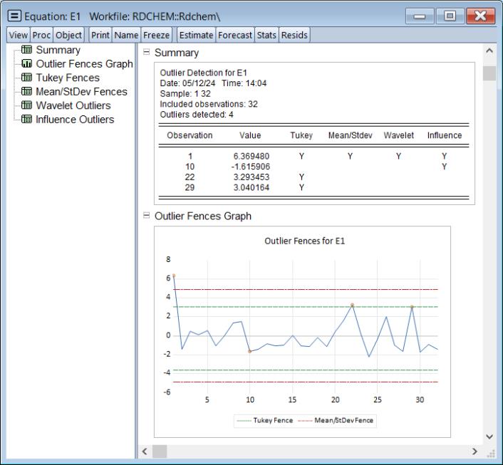
Series-based Outlier Detection
Outliers are observations in a series that significantly differ from the majority of the other observations. Whether due to measurement error, data entry mistakes, or simply natural variability in the data, outlier observations have values that stand out as unusual, rare, or abnormal when compared to the rest of the data.
The presence of outliers can have a substantial impact on statistical analysis, as outliers can skew statistical results and lead to inaccurate conclusions if not appropriately identified and handled.
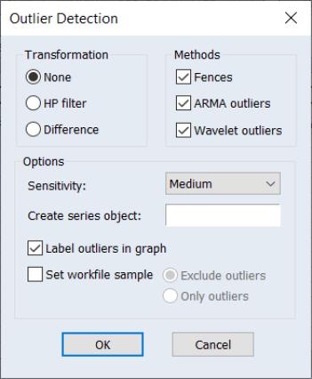
EViews 14 offers new easy-to-use tools for identifying outliers in a series or in the residuals of an estimated equation. You may use Tukey fences, mean/standard deviation fences, Wavelet outliers, and ARMA based outlier detection to identify outlier observations.
To perform outlier identification on observations in a single in EViews, open the series objctand click on View/Outlier Detection…. EViews will display the dialog:
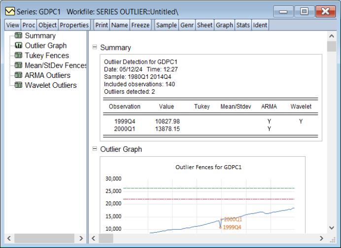
Filling out the dialog with the appropriate settings and clicking on produces a spool containing outlier identification tables and graphs:
• For discussion of the identification methods and examples, see the preliminary documentation in
“Outlier Detection”.
Equation-based Outlier Detection
The new outlier detection view of an equation performs various methods for detecting outliers associated with the equation estimates. This is a useful diagnostic tool to assess the validity of the model underlying the regression.
One set of equation outlier detection methods employs methods used to identify outliers in series (
“Outlier Detection”). A second set of equation outlier methods examines several of the influence statistics which measure the sensitivity of regression estimates to individual observations (
“Influence Statistics”) to determine whether an observation is an outlier. Observations which exhibit influence that exceeds a specified bound

are identified as outliers.
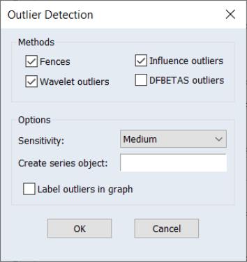
To perform outlier detection using the residuals from an equation in EViews, open the equation, and click on View/Outlier Diagnostics…. EViews will display the dialog:
The section offers checkboxes which select which of the outlier detection methods to use. The available options will depend on the method used to estimate the original equation.
• The and are only available for equations estimated by linear least squares.
• are only available for linear equations with ARMA terms.
When you click on OK, EViews will perform outlier identification using the specified methods and will display a spool containing both table and graphical results:
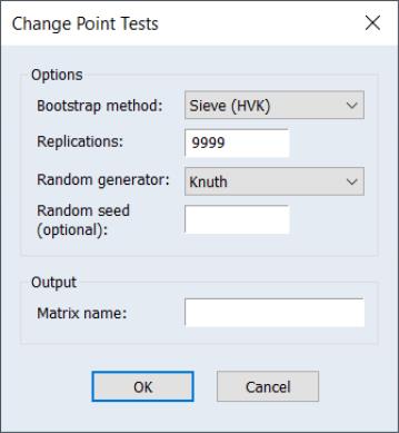
Break Testing and Change Point Detection
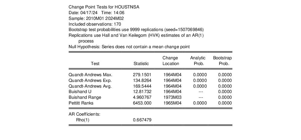
EViews 14 now computes Quandt-Andrews Regression, Pettitt Ranks, and a Buishand Range and U tests for a single change in the location parameter (mean) of a series, with optional bootstrapping of the test p-values.
Simply click on from the main series menu to display a dialog containing test and output settings:
You may use the dropdown menu to specify whether to compute bootstrap p-values, and if so, to select the bootstrap method. The remainder of the section provides options control the bootstrap computation. The section contains the Matrix name edit field for you to specify the name of a matrix object to store the test statistics and p-values.
The results of the change point tests are presented in a table:
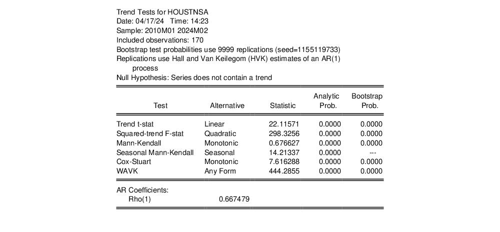
Trend Testing
Many economic time series follow a time-trend. Identification of the presence of trends is important, both for intrinsic interest and as a preliminary step for further econometric analysis.
EViews 14 includes parametric and non-parametric tests for the presence of a trend in a series. You may compute the linear trend t-test, the quadratic trend F-test, the Mann-Kendall test, Cox-Stuart test, and the Wang, Akritas, and Van Keilegon (WAVK) tests of a trend against various alternatives, with optional bootstrapping of the test p-values
To perform both trend tests on a series in EViews, click on from the main series menu:
You may use the dropdown menu to specify whether to compute bootstrap p-values, and if so, to select the bootstrap method. The remainder of the section provides options control the bootstrap computation. The section contains the Matrix name edit field for you to specify the name of a matrix object to store the test statistics and p-values.
The results of the change point tests are presented in a table:
Explosive Bubble Testing
Identification of bubbles in financial asset prices is an important topic in financial econometrics that has received considerable attention over the past decade (see Gürkaynak (2008) and Homm and Breitung (2012) for literature surveys).
EViews 14 offers Phillips et al.(2011, PWY) and Phillips et al. (2015, PSY) tests for detection of bubbles.
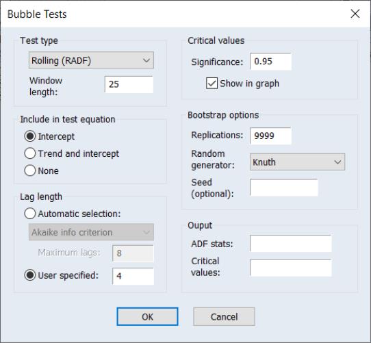
To perform a bubble test in EViews, open the series and click on View/Time Series Diagnostics/Bubble Tests…
The dialog offers choices for different test types, test equations, ADF lag lengths, and options for computing the bootstrap test probabilities and saving results to a matrix in the workfile.
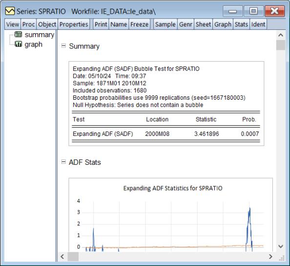
The output is in the form of a spool object containing a table showing the test results and a graph of the individual ADF statistics used in forming the test statistic.
Impulse Response Analysis
EViews 14 offers extensive additions and improvements to impulse response analysis of VARs and VECs, including impulse response via local projection and extensions of bootstrapping and monte carlo confidence intervals to additional models, and computation of Bayesian Time-varying Coefficient VAR fixed horizon impulse responses.
The new features include:
Impulse Response via Local Projection
The traditional VAR approach to impulse response estimation has both practical and theoretical shortcomings. In particular, the Wold decomposition can be difficult to derive, and may not exist, more likely in cases where the VAR is cointegrated. Further, impulse response functions derived from this method are justified only when the estimated VAR model coincides with the true DGP.
An alternative approach proposes the estimation of impulse responses via local projections (Jordà, 2005). The local projection (LP) technique is agnostic about the true DGP, and remains valid even when the Wold decomposition is undefined.
EViews 14 supports estimation of impulse responses via LP using both standard sequential and joint estimation. For sequential estimation, you may handle the serial correlation effect on covariance estimates using non-parametric HAC corrections.
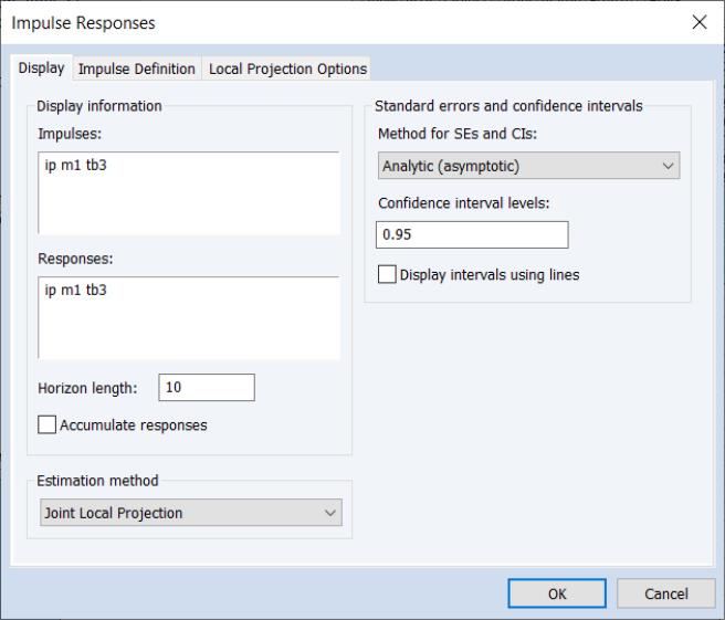
Do perform impulse response analysis using LP, press the Impulse button on the toolbar of an estimated VAR or click on to display the dialog. Then select either or in the impulse response dropdown menu:
Most of the settings in this dialog are familiar, controlling the impulses and responses to display, the horizon length, and the method of computing CIs. If you choose the monte carlo or bootstrap simulation methods you will be presented with additional options. EViews supports the bootstrap methods outlined by Jordà (2009) and Monteil Olea and Plagborg-Moller (2020)
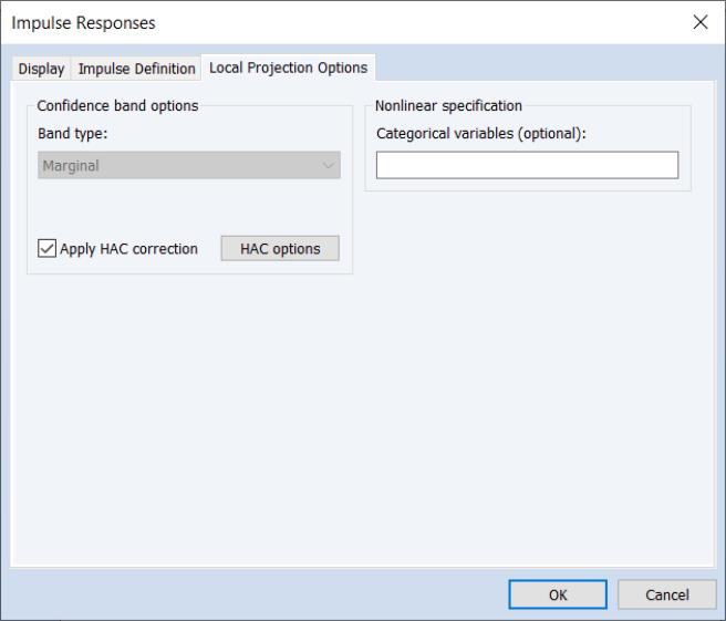
EViews will add a third tab to the dialog for setting . Click on the tab to make the dialog page active.
The settings will differ depending on whether you are estimating using sequential or joint LP. Here we see the settings for sequential projection, which offer us the option of accounting for serial correlation using HAC adjustment.
Note that non-linear/asymmetric LP may be specified by entering one or more categorical variables in the edit field.
Click on to compute the impulse responses and display the spool output:
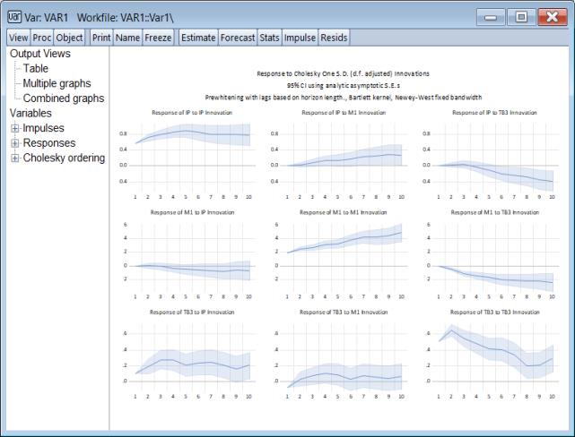
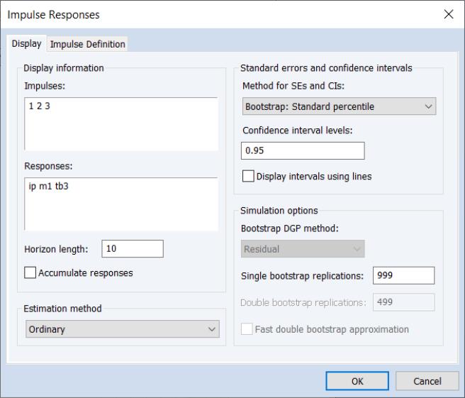
SVAR Impulse Response and Variance Decomposition CIs
Previous versions of EViews offered limited options for computing impulse response and variance decomposition CIs for structural VARS (SVARS). For impulse responses, CIs could only be computed using analytic or Monte Carlo methods; for variance decomposition, CIs and standard errors were unavailable.
EViews 14 can now perform Monte Carlo and bootstrap simulation for both SVAR impulse response and variance decomposition. If we press the button on the toolbar of an estimated SVAR or select from the menu, EViews will display the standard impulse response dialog:
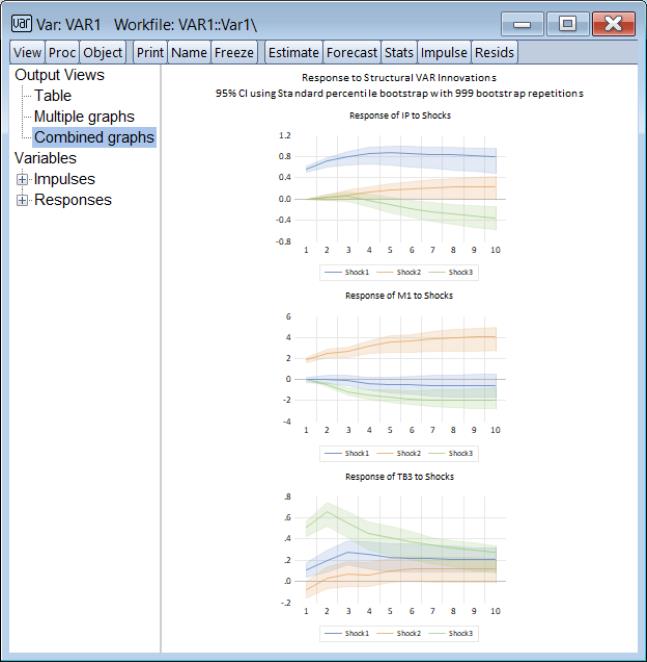
Importantly, the offers both Monte Carlo and a full set of bootstrap methods and options, even is you are working with a structural factorization:
Similar features are available for variance decomposition given a structural factorization.
Preliminary documentation is available:
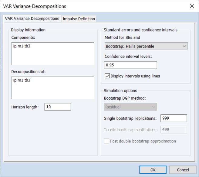
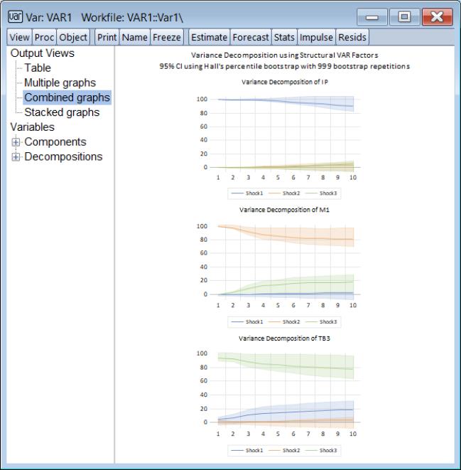
Variance Decomposition CIs
In prior versions of EViews, confidence intervals (CI) and standard errors (SEs) for variance decomposition were only available for reduced form VAR models and only via monte carlo simulation.
EViews 14 now offers its full suite of simulation-based CI methods for variance decomposition of both reduced form and structural models:
To perform the variance decomposition, select from the main menu of an estimated VAR.
You will be presented with a choice of . You may choose between none, Monte Carlo, and four different bootstrap methods, two of which feature a double bootstrap with optional fast double bootstrap algorithm. Depending on your choice, you will be presented with a variety of different options including the number of bootstrap replications.
Notably, all of these options are available, even if you elect to use structural impulses computed from the SVAR estimates..
Preliminary documentation is available:
BTVCVAR Fixed Horizon Impulse-Responses
EViews 14 offers powerful new tools for computing impulse-responses when working with the Bayesian time-varying VAR coefficients model.
The time-varying coefficient VAR (TVCVAR) relaxes the constant parameter restriction of conventional VARs, allowing for ongoing changes in model parameters over time. Unfortunately, allowing for time-varying coefficients exacerbates the problems associated with estimating VARs with large number of parameters.
Once estimated, the time-varying nature of coefficients introduce some complications into the analysis of the coefficients of the VAR notably in the analysis of impulse-responses.
Importantly, the TVCVAR impulse response is a function of both the timing (date) of the shock and the elapsed time since the shock. Timing matters for a TVCVAR because the VAR coefficients are different at different dates, so that the system responds differently to a given stimulus.
Prior versions of EViews produced tables and graphs of cross-sectional BTVCVAR IRFs at fixed dates. When performing impulse-response analysis, you were prompted to provide one or more dates at which to compute the IRFs, and a separate IRF was computed for each date.
EViews 14 offers new tools for producing BTVCVAR IRFs at fixed horizons, allowing you to examine how the system response at a given elapsed time has changed with changes in the impulse date. You will be prompted to provide one or more horizons, and EViews will compute the ensemble of IRFs and will extract and display the required results.
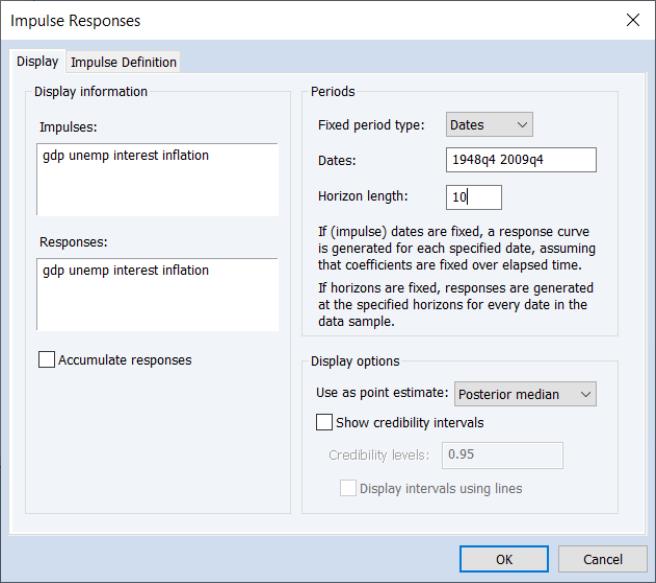
Click on the button on the toolbar of an estimated BTVCVAR or select from the menu, EViews will display the impulse response dialog:
You may use the to choose whether to display IRFs at different dates (), or do display IRFs collected at different horizons ().
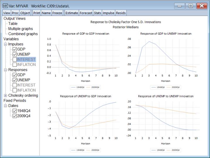
In the dialog depicted above we specify and ask for 10 period IRFs computed using the coefficients at two different dates (1948q4 and 2009q4):
Depicted are standard 10 period impulse responses for GDP and UNEMP for the two periods of interest.
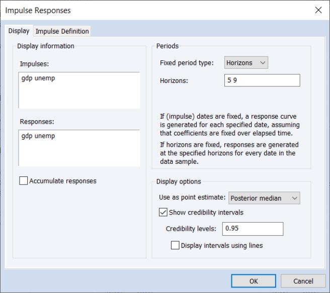
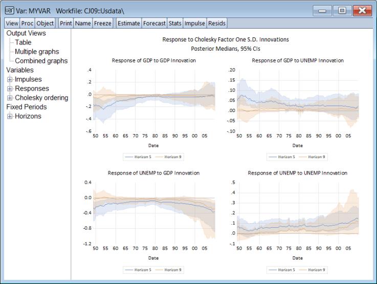
Alternately, we may specify and ask for the results of impulse responses computed at each period in the estimation sample for that horizon.
Here, we are asking EViews to compute the entire time-path of impulse responses at horizons of 5 and 9 periods:
Here we see the time-paths of the 5 and 9 horizon impulse responses for GDP and UNEMP.
For preliminary documentation:
• See
“Impulse Response” for further discussion of confidence interval computation and display in BTVCVAR models.
Matrix Statistical Tools
New Matrix Object Views and Procs
Prior versions of EViews offered somewhat limited statistical support for data held in vectors and matrices.
While basic statistical and mathematical functions like means and variances, mathematical function evaluation, and matrix algebra were all supported, a number of the analytic and utility views and procedures that were available for series and groups were not available for matrices and vectors. You could not, for example, easily test data in a vector for normality, or examine a one-way tabulation of the values in a vector.
In a number of settings, we found that having the ability to say, perform interactive analysis of data in a matrix or vector would be quite useful. While the matrix data could be exported to series or a new workfile, this was obviously inconvenient.
EViews 14 expands significantly the number of tools available for working with the data in vectors and matrices.
New Vector Views and Procs
For vectors you may now employ:
• histogram and stats view
• statistics by classification view
• one-way frequency tables
• parametric and non-parametric measures of variability
• simple hypothesis tests
• equality tests by classification
• empirical distribution tests
• resampling
• creating classification vectors
• making distribution function data (for example, saving kernel density data)
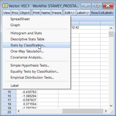
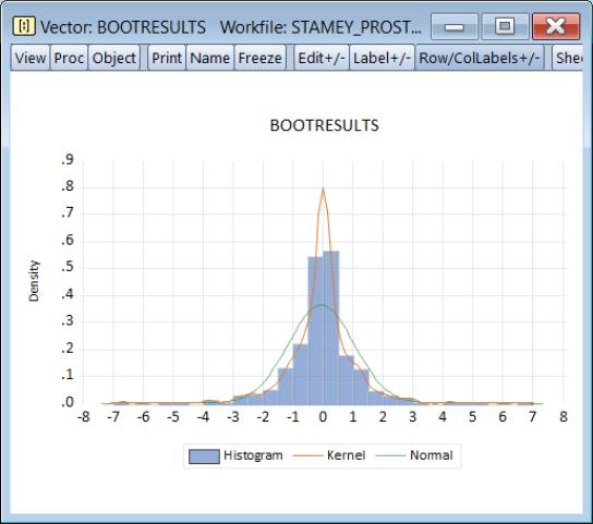
For example, if you have results from a bootstrap simulation stored in a vector, it is now easy to produce both a custom distribution graph,
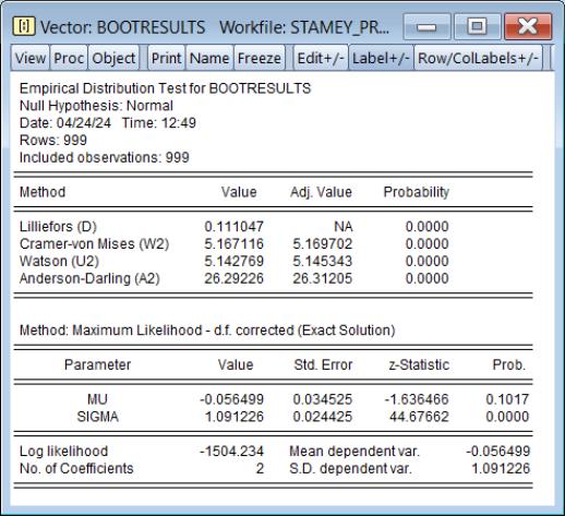
and perform empirical distribution function tests
For updated command documentation see:
Vector / Rowvector
classify recode vector into classes defined by a grid, specified limits, or quantiles.
distdata save a matrix containing distribution plot data computed from the series.
edftest empirical distribution function tests.
hist descriptive statistics and histogram.
resample resample from the observations in the vector
.
statby statistics by classification.
stats descriptive statistics of the data in the vector.
testby equality test by classification.
Svector
New Matrix Views and Procs
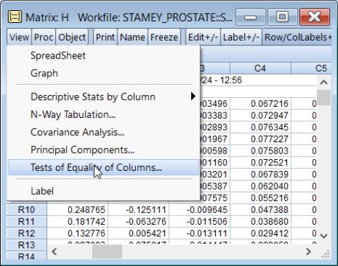
Similarly, for matrices, you may now perform:
• descriptive statistics
• n-way cross-tabulation
• tests of equality of column statistics
• resampling from the rows of the matrix
• making distribution function data
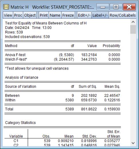
For example, we can test for equality of the means between the columns of a matrix,
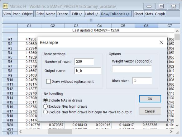
and resample from the rows of the matrix
For updated command documentation see:
distdata save a matrix containing distribution plot data computed from the matrix.
freq 
-way contingency table.
resample resample from rows of the matrix .
stats descriptive statistics for each column of the matrix.
testbtw tests of equality for mean, median, or variance between series in group.